N-dimensional reductions with Blosc2

NumPy is widely recognized for its ability to perform efficient computations and manipulations on multidimensional arrays. This library is fundamental for many aspects of data analysis and science due to its speed and flexibility in handling numerical data. However, when datasets reach considerable sizes, working with uncompressed data can result in prolonged access times and intensive memory usage, which can negatively impact overall performance.

Python-Blosc2 leverages the power of NumPy to perform reductions on compressed multidimensional arrays. But, by compressing data with Blosc2, it is possible to reduce the memory and storage space required to store large datasets, while maintaining fast reduction times. This is especially beneficial for systems with memory constraints, as it allows for faster data access and operation.

In this blog, we will explore how Python-Blosc2 can perform data reductions in in-memory NDArray objects (or any other object fulfilling the LazyArray interface) and how the speed of these operations can be optimized by using different chunk shapes, compression levels and codecs. We will then compare the performance of Python-Blosc2 with NumPy.

Note: The code snippets shown in this blog are part of a Jupyter notebook that you can run on your own machine. For that, you will need to install a recent version of Python-Blosc2: pip install 'blosc2>=3.0.0b3'; feel free to experiment with different parameters and share your results with us!

The 3D array

We will use a 3D array of type float64 with shape (1000, 1000, 1000). This array will be filled with values from 0 to 1000, and the goal will be to compute the sum of values in stripes of 100 elements in one axis, and including all the values in the other axis. We will perform reductions along the X, Y, and Z axes, comparing Blosc2 performance (with and without compression) against NumPy.

Reducing with NumPy

We will start by performing different sum reductions using NumPy. First, summing along the X, Y, and Z axes (and getting 2D arrays as result) and then summing along all axis (and getting an scalar as result).

axes = ("X", "Y", "Z", "all")
meas_np = {"sum": {}, "time": {}}
for n, axis in enumerate(axes):
    n = n if axis != "all" else None
    t0 = time()
    meas_np["sum"][axis] = np.sum(a, axis=n)
    t = time() - t0
    meas_np["time"][axis] = time() - t0

Reducing with Blosc2

Now let's create the Blosc2 array from the NumPy array. First, let's define the parameters for Blosc2: number of threads, compression levels, codecs, and chunk sizes. We will exercise different combinations of these parameters (including no compression) to evaluate the performance of Python-Blosc2 in reducing data in 3D arrays.

# Params for Blosc2
clevels = (0, 5)
codecs = (blosc2.Codec.LZ4, blosc2.Codec.ZSTD)

The function shown below is responsible for creating the different arrays and performing the reductions for each combination of parameters.

# Create a 3D array of type float64
def measure_blosc2(chunks):
    meas = {}
    for codec in codecs:
        meas[codec] = {}
        for clevel in clevels:
            meas[codec][clevel] = {"sum": {}, "time": {}}
            cparams = {"clevel": clevel, "codec": codec}
            a1 = blosc2.asarray(a, chunks=chunks, cparams=cparams)
            if clevel > 0:
                print(f"cratio for {codec.name} + SHUFFLE: {a1.schunk.cratio:.1f}x")
            # Iterate on Blosc2 and NumPy arrays
            for n, axis in enumerate(axes):
                n = n if axis != "all" else None
                t0 = time()
                # Perform the sum of the stripe (defined by the slice_)
                meas[codec][clevel]["sum"][axis] = a1.sum(axis=n)
                t = time() - t0
                meas[codec][clevel]["time"][axis] = t
                # If interested, you can uncomment the following line to check the results
                #np.testing.assert_allclose(meas[codec][clevel]["sum"][axis],
                #                           meas_np["sum"][axis])
    return meas

Automatic chunking

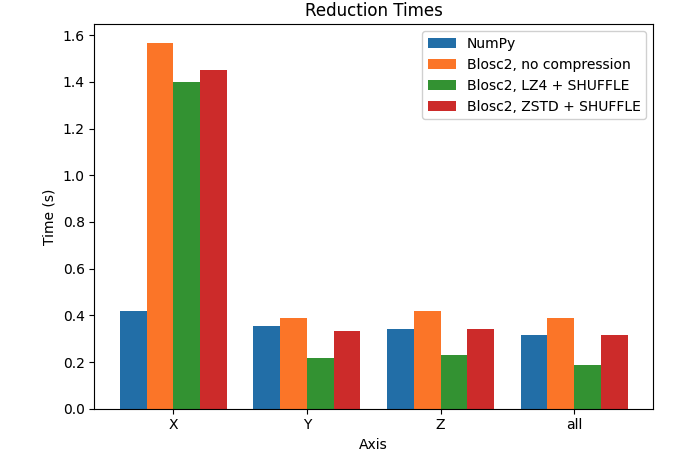
Let's plot the results for the X, Y, and Z axes, comparing the performance of Python-Blosc2 with different configurations against NumPy.

/images/ndim-reductions/plot_automatic_chunking.png

We can see that reduction along the X axis is much slower than those along the Y and Z axis for the Blosc2 case. This is because the automatically computed chunk shape is (1, 1000, 1000) making the overhead of partial sums larger. In addition, we see that, when reducing in all axes, as well as in Y and Z axes, Blosc2+LZ4+SHUFFLE actually achieves far better performance than NumPy. Finally, when not using compression inside Blosc2, we never see an advantage. See later for a discussion on these results.

Manual chunking

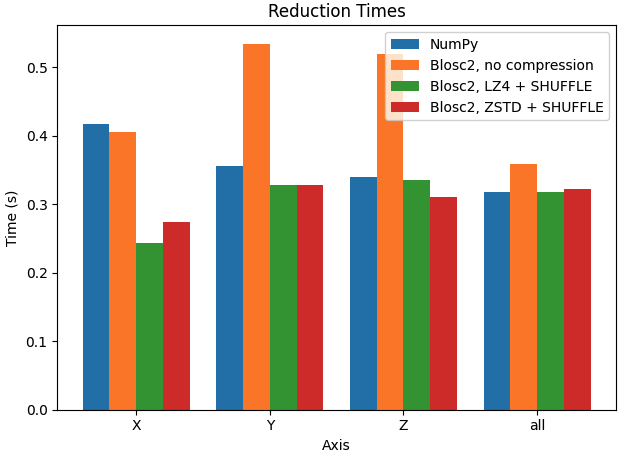
Let's try to improve the performance by manually setting the chunk size. In the next case, we want to make performance similar along the three axes, so we will set the chunk size to (100, 100, 100) (8 MB).

/images/ndim-reductions/plot_manual_chunking.png

In this case, performance in the X axis is already faster than Y and Z axes for Blosc2. Interestingly, performance is also faster than NumPy in X axis, while being very similar in Y and Z axis.

We could proceed further and try to fine tune the chunk size to get even better performance, but this is out of the scope of this blog (and more a task for Btune). Instead, we will try to make some sense on the results above; see below.

Why Blosc2 can be faster than NumPy?

As Blosc2 is using the NumPy machinery for computing reductions behind the scenes, why is Blosc2 faster than NumPy in several cases above? The answer lies in the way Blosc2 and NumPy access data in memory.

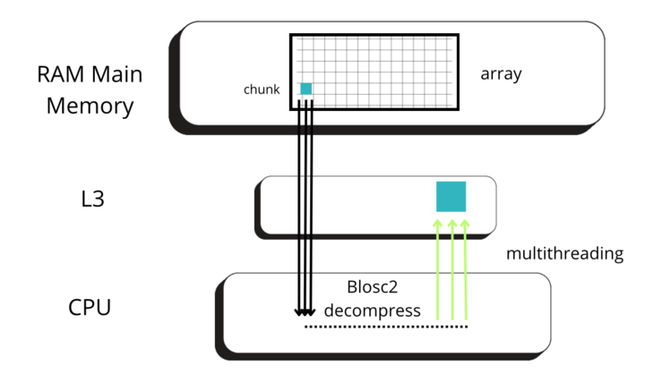
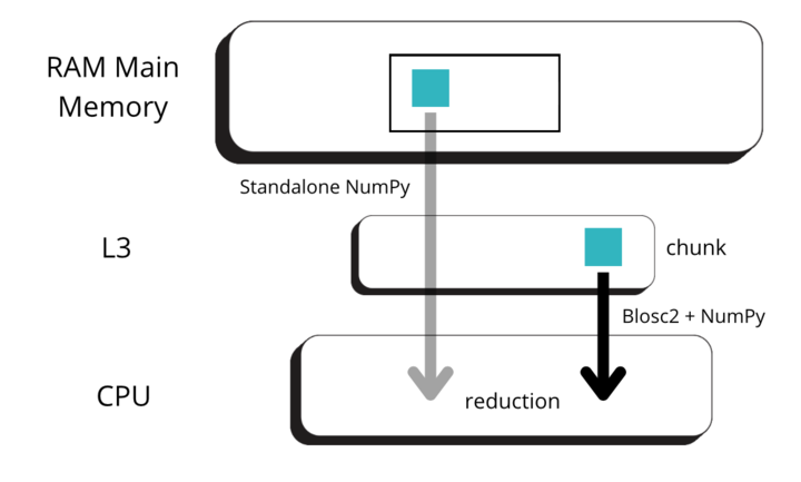
Blosc2 splits data into chunks and blocks to compress and decompress data efficiently. When accessing data, a full chunk is fetched from memory and decompressed by the CPU (as seen in the image below, left side). If the chunk size is small enough to fit in the CPU cache, the CPU can write the decompressed chunk faster, as it does not need to travel back to the main memory. Later, when NumPy is called to perform the reduction on the decompressed chunk, it can access the data faster, as it is already in the CPU cache (image below, right side).

/images/ndim-reductions/Blosc2-decompress.png /images/ndim-reductions/Blosc2-NumPy.png

But for allowing NumPy go faster, Blosc2 needs to decompress several chunks prior to NumPy performing the reduction operation. The decompressed chunks are stored on a queue, waiting for further processing; this is why Blosc2 needs to handle several (3 or 4) chunks simultaneously. In our case, the L3 cache size of our CPU (Intel 13900K) is 36 MB, and Blosc2 has chosen 8 MB for the chunk size, allowing to store up to 4 chunks in L3, which is near to optimal. Also, when we have chosen the chunk size to be (100, 100, 100), the chunk size is still 8 MB, which continues to be fine indeed.

All in all, it is not that Blosc2 is faster than NumPy, but rather that it is allowing NumPy to leverage the CPU cache more efficiently. Having said this, we still need some explanation on why the performance can be so different along the X, Y, and Z axes, specially for the first chunk shape (automatic) above. Let's address this in the next section.

Performing reductions on 3D arrays

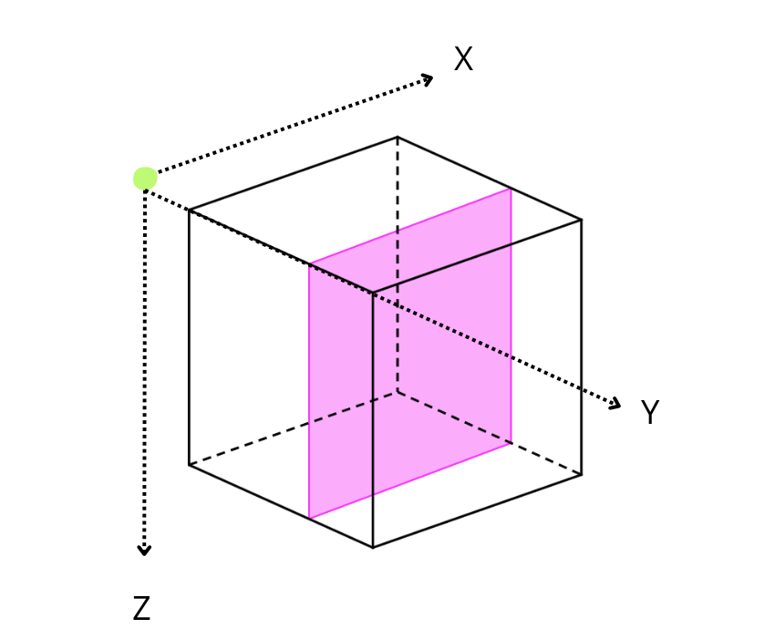
/images/ndim-reductions/3D-cube-plane.png

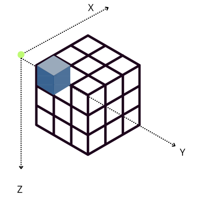
On a three-dimensional environment, like the one shown in the image, data is organized in a cubic space with three axes: X, Y, and Z. By default, Blosc2 chooses the chunk size so that it fits in the CPU cache comfortably. On the other hand, it tries to follow the NumPy convention of storing data row-wise; so, this is why the default chunk shape has been chosen as (1, 1000, 1000). In this case, it is clear that reduction times along different axes are not going to be the same, as the sizes of the chunk in different axes are not uniform (actually, there is a large asymmetry).

The difference in cost while traversing data values can be visualized more easily on a 2D array:

/images/ndim-reductions/memory-access-2D-x.png

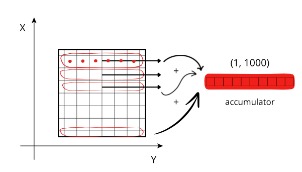
Reduction along the X axis: When accessing a row (red line), the CPU can access these values (red points) from memory sequentially, but they need to be stored on an accumulator. The next rows needs to be fetched from memory and be added to the accumulator. If the size of the accumulator is large (in this case is 1000 * 1000 * 8 = 8 MB), it does not fit in low level CPU caches, and has to be peformed in the relatively slow L3.

/images/ndim-reductions/memory-access-2D-y.png

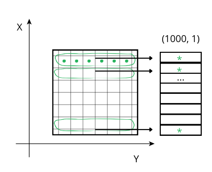
Reducing along the Y axis: When accessing a row (green line), the CPU can access these values (green points) from memory sequentially but, contrarily to the case above, they don't even need an accumulator, and the sum of the row (marked as an *) is final. So, although the number of sum operations is the same as above, the required time is smaller because there is no need of updating all the values of the accumulator per row, but only one at a time, which is faster in modern CPUs.

Tweaking the chunk size

/images/ndim-reductions/3D-cube.png

However, when Blosc2 is instructed to create chunks that are the same size for all the axes (chunks=(100, 100, 100)), the situation changes. In this case, an accumulator is needed for each chunk (sub-cube in figure above), but as it is relatively small (100 * 100 * 8 = 80 KB), and fits in L2, so accumulation in the X axis is faster than in the previous scenario (remember that it needs to do the accumulation in L3).

Incidentally, now Blosc2 performance along X axis is even better than in the Y and Z axes, as the CPU can access data in a more efficient way. Furthermore, Blosc2 performance is up to 1.5x better than NumPy in the X axis (while being similar, or even a bit better along Y and Z axes), which is a quite remarkable feat.

Effect of using different codecs in Python-Blosc2

Compression and decompression consume CPU and memory resources. Differentiating between various codecs and configurations allows for evaluating how each option impacts the use of these resources, helping to choose the most efficient option for the operating environment. Finding the right balance between compression ratio and speed is crucial for optimizing performance.

In the plots above, we can see how using the LZ4 codec is striking such a balance, as it achieves the best performance in general, even above a non-compressed scenario. This is because LZ4 is tuned towards speed, and the time to compress and decompress the data is very low. On the other hand, ZSTD is a codec that is optimized for compression ratio (although not shown, in this case it typically compresses between 2x and x more than LZ4), and hence it is a bit slower. However, it is still faster than the non-compressed case, as compression requires reduced memory transmission, and this compensates for the additional CPU time required for compression and decompression.

We have just scraped the surface for some of the compression parameters that can be tuned in Blosc2. You can use the cparams dict with the different parameters in blosc2.compress2() to set the compression level, codec , filters and other parameters.

Conclusion

Understanding the balance between space savings and the additional time required to process the data is important. Testing different compression settings can help finding the method that offers the best trade-off between reduced size and processing time. The fact that Blosc2 automatically chooses the chunk shape, makes it easy for the user to get a decently good performance, without having to worry about the details of the CPU cache. In addition, as we have shown, we can fine tune the chunk shape in case the default one does not fit our needs (e.g. we need more uniform performance along all axes).

Besides the sum() reduction exercised here, Blosc2 supports a fair range of reduction operators (mean, std, min, max, all, any, etc.), and you are invited to explore them. Moreover, it is also possible to use reductions even for very large arrays that are stored on disk. This opens the door to a wide range of possibilities for data analysis and science, allowing for efficient reductions on large datasets that are compressed on-disk and with minimal memory usage. We will explore this in a forthcoming blog.

We would like to thank ironArray for supporting the development of the computing capabilities of Blosc2. Then, to NumFOCUS for recently providing a small grant that is helping us to improve the documentation for the project. Last but not least, we would like to thank the Blosc community for providing so many valuable insights and feedback that have helped us to improve the performance and usability of Blosc2.

Peaking compression performance in PyTables with direct chunking

It took a while to put things together, but after many months of hard work by maintainers, developers and contributors, PyTables 3.10 finally saw the light, full of enhancements and fixes. Thanks to a NumFOCUS Small Development Grant, we were able to include a new feature that can help you squeeze considerable performance improvements when using compression: the direct chunking API.

In a previous post about optimized slicing we saw the advantages of avoiding the overhead introduced by the HDF5 filter pipeline, in particular when working with multi-dimensional arrays compressed with Blosc2. This is achieved by specialized, low-level code in PyTables which understands the structure of the compressed data in each chunk and accesses it directly, with the least possible intervention of the HDF5 library.

However, there are many reasons to exploit direct chunk access in your own code, from customizing compression with parameters not allowed by the PyTables Filters class, to using yet-unsupported compressors or even helping you develop new plugins for HDF5 to support them (you may write compressed chunks in Python while decompressing transparently in a C filter plugin, or vice versa). And of course, as we will see, skipping the HDF5 filter pipeline with direct chunking may be instrumental to reach the extreme I/O performance required in scenarios like continuous collection or extraction of data.

PyTables' new direct chunking API is the machinery that gives you access to these possibilities. Keep in mind though that this is a low-level functionality that may help you largely customize and accelerate access to your datasets, but may also break them. In this post we'll try to show how to use it to get the best results.

Using the API

The direct chunking API consists of three operations: get information about a chunk (chunk_info()), write a raw chunk (write_chunk()), and read a raw chunk (read_chunk()). They are supported by chunked datasets (CArray, EArray and Table), i.e. those whose data is split into fixed-size chunks of the same dimensionality as the dataset (maybe padded at its boundaries), with HDF5 pipeline filters like compressors optionally processing them on read/write.

chunk_info() returns an object with useful information about the chunk containing the item at the given coordinates. Let's create a simple 100x100 array with 10x100 chunks compressed with Blosc2+LZ4 and get info about a chunk:

>>> import tables, numpy
>>> h5f = tables.open_file('direct-example.h5', mode='w')
>>> filters = tables.Filters(complib='blosc2:lz4', complevel=2)
>>> data = numpy.arange(100 * 100).reshape((100, 100))
>>> carray = h5f.create_carray('/', 'carray', chunkshape=(10, 100),
                               obj=data, filters=filters)
>>> coords = (42, 23)
>>> cinfo = carray.chunk_info(coords)
>>> cinfo
ChunkInfo(start=(40, 0), filter_mask=0, offset=6779, size=608)

So the item at coordinates (42, 23) is stored in a chunk of 608 bytes (compressed) which starts at coordinates (40, 0) in the array and byte 6779 in the file. The latter offset may be used to let other code access the chunk directly on storage. For instance, since Blosc2 was the only HDF5 filter used to process the chunk, let's open it directly:

>>> import blosc2
>>> h5f.flush()
>>> b2chunk = blosc2.open(h5f.filename, mode='r', offset=cinfo.offset)
>>> b2chunk.shape, b2chunk.dtype, data.itemsize
((10, 100), dtype('V8'), 8)

Since Blosc2 does understand the structure of data (thanks to b2nd), we can even see that the chunk shape and the data item size are correct. The data type is opaque to the HDF5 filter which wrote the chunk, hence the V8 dtype. Let's check that the item at (42, 23) is indeed in that chunk:

>>> chunk = numpy.ndarray(b2chunk.shape, buffer=b2chunk[:],
                          dtype=data.dtype)  # Use the right type.
>>> ccoords = tuple(numpy.subtract(coords, cinfo.start))
>>> bool(data[coords] == chunk[ccoords])
True

This offset-based access is actually what b2nd optimized slicing performs internally. Please note that neither PyTables nor HDF5 were involved at all in the actual reading of the chunk (Blosc2 just got a file name and an offset). It's difficult to cut more overhead than that!

It won't always be the case that you can (or want to) read a chunk in that way. The read_chunk() method allows you to read a raw chunk as a new byte string or into an existing buffer, given the chunk's start coordinates (which you may compute yourself or get via chunk_info()). Let's use read_chunk() to redo the reading that we just did above:

>>> rchunk = carray.read_chunk(coords)
Traceback (most recent call last):
    ...
tables.exceptions.NotChunkAlignedError: Coordinates are not multiples
    of chunk shape: (42, 23) !* (np.int64(10), np.int64(100))
>>> rchunk = carray.read_chunk(cinfo.start)  # Always use chunk start!
>>> b2chunk = blosc2.ndarray_from_cframe(rchunk)
>>> chunk = numpy.ndarray(b2chunk.shape, buffer=b2chunk[:],
                          dtype=data.dtype)  # Use the right type.
>>> bool(data[coords] == chunk[ccoords])
True

The write_chunk() method allows you to write a byte string into a raw chunk. Please note that you must first apply any filters manually, and that you can't write chunks beyond the dataset's current shape. However, remember that enlargeable datasets may be grown or shrunk in an efficient manner using the truncate() method, which doesn't write new chunk data. Let's use that to create an EArray with the same data as the previous CArray, chunk by chunk:

>>> earray = h5f.create_earray('/', 'earray', chunkshape=carray.chunkshape,
                               atom=carray.atom, shape=(0, 100),  # Empty.
                               filters=filters)  # Just to hint readers.
>>> earray.write_chunk((0, 0), b'whatever')
Traceback (most recent call last):
    ...
IndexError: Chunk coordinates not within dataset shape:
    (0, 0) <> (np.int64(0), np.int64(100))
>>> earray.truncate(len(carray))  # Grow the array (cheaply) first!
>>> for cstart in range(0, len(carray), carray.chunkshape[0]):
...     chunk = carray[cstart:cstart + carray.chunkshape[0]]
...     b2chunk = blosc2.asarray(chunk)  # May be customized.
...     wchunk = b2chunk.to_cframe()  # Serialize.
...     earray.write_chunk((cstart, 0), wchunk)

You can see that such low-level writing is more involved than usual. Though we used default Blosc2 parameters here, the explicit compression step allows you to fine-tune it in ways not available through PyTables like setting internal chunk and block sizes or even using Blosc2 compression plugins like Grok/JPEG2000. In fact, the filters given on dataset creation are only used as a hint, since each Blosc2 container holding a chunk includes enough metadata to process it independently. In the example, the default chunk compression parameters don't even match dataset filters (using Zstd instead of LZ4):

>>> carray.filters
Filters(complevel=2, complib='blosc2:lz4', ...)
>>> earray.filters
Filters(complevel=2, complib='blosc2:lz4', ...)
>>> b2chunk.schunk.cparams['codec']
<Codec.ZSTD: 5>

Still, the Blosc2 HDF5 filter plugin included with PyTables is able to read the data just fine:

>>> bool((carray[:] == earray[:]).all())
True
>>> h5f.close()

You may find a more elaborate example of using direct chunking in PyTables' examples.

Benchmarks

b2nd optimized slicing shows us that removing the HDF5 filter pipeline from the I/O path can result in sizable performance increases, if the right chunking and compression parameters are chosen. To check the impact of using the new direct chunking API, we ran some benchmarks that compare regular and direct read/write speeds. On an AMD Ryzen 7 7800X3D CPU with 8 cores, 96 MB L3 cache and 8 MB L2 cache, clocked at 4.2 GHz, we got the following results:

/images/pytables-direct-chunking/AMD-7800X3D.png

We can see that direct chunking yields 3.75x write and 4.4x read speedups, reaching write/read speeds of 1.7 GB/s and 5.2 GB/s. These are quite impressive numbers, though the base equipment is already quite powerful. Thus we also tried the same benchmark on a consumer-level MacBook Air laptop with an Apple M1 CPU with 4+4 cores and 12 MB L2 cache, clocked at 3.2 GHz, with the following results:

/images/pytables-direct-chunking/MacAir-M1.png

In this case direct chunking yields 4.5x write and 1.9x read speedups, with write/read speeds of 0.8 GB/s and 1.6 GB/s. The absolute numbers are of course not as impressive, but the performance is still much better than that of the regular mechanism, especially when writing. Please note that the M1 CPU has a hybrid efficiency+performance core configuration; as an aside, running the benchmark on a high-range Intel Core i9-13900K CPU also with a hybrid 8+16 core configuration (32 MB L2, 5.7 GHz) raised the write speedup to 4.6x, reaching an awesome write speed of 2.6 GB/s.

All in all, it's clear that bypassing the HDF5 filter pipeline results in immediate I/O speedups. You may find a Jupyter notebook with the benchmark code and AMD CPU data in PyTables' benchmarks.

Conclusions

First of all, we (Ivan Vilata and Francesc Alted) want to thank everyone who made this new 3.10 release of PyTables possible, especially Antonio Valentino for his role of project maintainer, and the many code and issue contributors. Trying the new direct chunking API is much easier because of them. And of course, a big thank you to the NumFOCUS Foundation for making this whole new feature possible by funding its development!

In this post we saw how PyTables' direct chunking API allows one to squeeze the extra drop of performance that the most demanding scenarios require, when adjusting chunking and compression parameters in PyTables itself can't go any further. Of course, its low-level nature makes its use less convenient and safe than higher-level mechanisms, so you should evaluate whether the extra effort pays off. If used carefully with robust filters like Blosc2, the direct chunking API should shine the most in the case of large datasets with sustained I/O throughput demands, while retaining compatibility with other HDF5-based tools.

Exploring lossy compression with Blosc2

In the realm of data compression, efficiency is key. Whether you're dealing with massive datasets or simply aiming to optimize storage space and transmission speeds, the choice of compression algorithm can make a significant difference. In this blog post, we'll delve into the world of lossy compression using Blosc2, exploring its capabilities, advantages, and potential applications.

Understanding lossy compression

Unlike lossless compression, where the original data can be perfectly reconstructed from the compressed version, lossy compression involves discarding some information to achieve higher compression ratios. While this inevitably results in a loss of fidelity, the trade-off is often justified by the significant reduction in storage size.

Lossy compression techniques are commonly employed in scenarios where minor degradation in quality is acceptable, such as multimedia applications (e.g., images, audio, and video) and scientific data analysis. By intelligently discarding less crucial information, lossy compression algorithms can achieve substantial compression ratios while maintaining perceptual quality within acceptable bounds.

Lossy codecs in Blosc2

In the context of Blosc2, lossy compression can be achieved either through a combination of traditional compression algorithms and filters that can selectively discard less critical data, or by using codecs specially meant for doing so.

Filters for truncating precision

Since its inception, Blosc2 has featured the TRUNC_PREC filter, which is meant to discard the least significant bits from floating-point values (be they float32 or float64). This filter operates by zeroing out the designated bits slated for removal, resulting in enhanced compression. To see the impact on compression ratio and speed, an illustrative example here.

A particularly useful use case of the TRUNC_PREC filter is to truncate precision of float32/float64 types to either 8 or 16 bit; this is a quick and dirty way to ‘fake’ float8 or float16 types, which are very much used in AI nowadays, and contain storage needs.

In that vein, we recently implemented the INT_TRUNC filter, which does the same as TRUNC_PREC, but for integers (int8, int16, int32 and int64, and their unsigned counterparts). With both TRUNC_PREC and INT_TRUNC, you can specify an acceptable precision for most numerical data types.

Codecs for NDim datasets

Blosc2 has support for ZFP, another codec that is very useful for compressing multidimensional datasets. Although ZFP itself supports both lossless and lossy compression, Blosc2 makes use of its lossy capabilities only (the lossless ones are supposed to be already covered by other codecs in Blosc2). See this blog post for more info on the kind of lossy compression that can be achieved with ZFP.

Codecs for images

In addition, we recently included support for a couple of codecs that support the JPEG 2000 standard. One is OpenJ2HK, and the other is grok. Both have good, high quality JPEG 2000 implementations, but grok is a bit more advanced and has support for 16-bit gray images; we have blogged about it.

Experimental filters

Finally, you may want to experiment with some filters and codecs that were mainly designed to be a learning tool for people wanting to implement their own ones. Among them you can find:

  • NDCELL: A filter that groups data in multidimensional cells, reordering them so that the codec can find better repetition patterns on a cell-by-cell basis.

  • NDMEAN: A multidimensional filter for lossy compression in multidimensional cells, replacing all elements in a cell by the mean of the cell. This allows for better compressions by the actual compression codec (e.g. NDLZ).

  • NDLZ: A compressor based on the Lempel-Ziv algorithm for 2-dim datasets. Although this is a lossless compressor, it is actually meant to be used in combination with the NDCELL and NDMEAN above, providing lossy compression for the latter case.

Again, the codecs in this section are not specially efficient, but can be used for learning about the compression pipeline in Blosc2. For more info on how to implement (and register) your own filters, see this blog post.

Applications and use cases

The versatility of Blosc2's lossy compression capabilities opens up a myriad of applications across different domains. In scientific computing, for example, where large volumes of data are generated and analyzed, lossy compression can significantly reduce storage requirements without significantly impacting the accuracy of results.

Similarly, in multimedia applications, such as image and video processing, lossy compression can help minimize bandwidth usage and storage costs while maintaining perceptual quality within acceptable limits.

Compressing images with JPEG 2000 and with INT_TRUNC

As an illustration, a recent study involved the compression of substantial volumes of 16-bit grayscale images sourced from different synchrotron facilities in Europe. While achieving efficient compression ratios necessitates the use of lossy compression techniques, it is essential to exercise caution to preserve key features for clear visual examination and accurate numerical analysis. Below, we provide an overview of how Blosc2 can employ various codecs and quality settings within filters to accomplish this task.

Lossy compression (quality)

The SSIM index, derived from the Structural Similarity Measure, gauges the perceived quality of an image, with values closer to 1 indicating higher fidelity. You can appreciate the varying levels of fidelity achievable through the utilization of different filters and codecs.

In terms of performance, each of these compression methods also showcases significantly varied speeds (tested on a MacBook Air with an M1 processor):

Lossy compression (speed)

A pivotal benefit of Blosc2's strategy for lossy compression lies in its adaptability and configurability. This enables tailoring to unique needs and limitations, guaranteeing optimal performance across various scenarios.

Using Blosc2 within HDF5

HDF5 is a widely used data format, and both major Python wrappers, h5py (via hdf5plugin) and PyTables, offer basic support for Blosc2. However, accessing the full capabilities of the Blosc2 compression pipeline is somewhat restricted because the current hdf5-blosc2 filter, available in PyTables (and used by hdf5plugin), is not yet equipped to transmit all the necessary parameters to the HDF5 data pipeline.

Thankfully, HDF5 includes support for the direct chunking mechanism, which enables the direct transmission of pre-compressed chunks to HDF5, bypassing its standard data pipeline. Since h5py also offers this functionality, it's entirely feasible to leverage all the advanced features of Blosc2, including lossy compression. Below are a couple of examples illustrating how this process operates:

Conclusion

Lossy compression is a powerful tool for optimizing storage space, reducing bandwidth usage, and improving overall efficiency in data handling. With Blosc2, developers have access to a robust and flexible compression library for both lossless and lossy compression modes.

With its advanced compression methodologies and adept memory management, Blosc2 empowers users to strike a harmonious balance between compression ratio, speed, and fidelity. This attribute renders it especially suitable for scenarios where resource limitations or performance considerations hold significant weight.

Finally, there are ongoing efforts towards integrating fidelity into our BTune AI tool. This enhancement will empower the tool to autonomously identify the most suitable codecs and filters, balancing compression level, precision, and fidelity according to user-defined preferences. Keep an eye out for updates!

Whether you're working with scientific data, multimedia content, or large-scale datasets, Blosc2 offers a comprehensive solution for efficient data compression and handling.

Special thanks to sponsors and developers

Gratitude goes out to our sponsors over the years, with special recognition to the LEAPS collaboration and NumFOCUS, whose support has been instrumental in advancing the lossy compression capabilities within Blosc2.

The Blosc2 project is the outcome of the work of many developers.

New grok plugin for Blosc2

Update 2024-01-04: Use the new global plugin ID for the grok codec in the examples.

The Blosc Development Team is happy to announce that the first public release (0.2.0) of blosc2-grok is available for testing. This dynamic plugin is meant for using the JPEG2000 codec from the grok library as another codec inside Blosc2 (both from C and Python).

In this blog we will see how to use it as well as the functionality of some parameters. To do so, we will depict an already created example. Let's get started!

Why JPEG2000?

It can be stated that currently the best compromise between image quality and compression factor is JPEG2000. This image compression standard has been in use for over 20 years and is widely accepted in the imaging community due to its ability to achieve a compression factor of approximately 10x without significant loss of information.

JPEG2000 has been implemented in many libraries, but the one that stands out is the grok library because of its speed and completeness. This is why we have chosen it to be the first image codec to be added to Blosc2.

Installing the plugin

First of all, you will need to install the blosc2-grok plugin. You can do it with:

pip install blosc2-grok

That's it! You are ready to use it.

Using the grok codec via the plugin

The grok codec has been already registered as a global plugin for Blosc2, so you only need to use its plugin id (blosc2.Codec.GROK) in the codec field of the cparams:

# Define the compression parameters. Disable the filters and the
# splitmode, because these don't work with the codec.
cparams = {
    'codec': blosc2.Codec.GROK,
    'filters': [],
    'splitmode': blosc2.SplitMode.NEVER_SPLIT,
}

It is important to disable any filter or splitmode, since we don't want the data to be modified before proceeding to the compression using grok.

Now, imagine you have an image as a NumPy array (let's say, created using pillow), and you want to compress via blosc2_grok. Before, you will need to tell blosc2-grok which format to use among the available ones in the grok library (we will get through the different parameters later):

# Set the parameters that will be used by the codec
kwargs = {'cod_format': blosc2_grok.GrkFileFmt.GRK_FMT_JP2}
blosc2_grok.set_params_defaults(**kwargs)

And finally, you are able to compress the image with:

bl_array = blosc2.asarray(
    np_array,
    chunks=np_array.shape,
    blocks=np_array.shape,
    cparams=cparams,
    urlpath="myfile.b2nd",
    mode="w",
)

We already have compressed our first image with blosc2-grok!

In this case, the chunks and blocks params of Blosc2 have been set to the shape of the image (including the number of components) so that grok receives the image as a whole and therefore, can find more opportunities to compress better.

Setting grok parameters

We have already used the cod_format grok parameter to set the format to use with the blosc2_grok.set_params_defaults(), but blosc2-grok lets you set many other parameters. All of them are mentioned in the README. When possible, and to make it easier for existing users, these parameters are named the same than in the Pillow library.

For example, let's see how to set the quality_mode and quality_layers params, which are meant for lossy compression. So, realize you don't care too much about the quality but want a compression ratio of 10x. Then, you would specify the quality_mode to be rates and the quality_layers to 10:

kwargs = {'cod_format': blosc2_grok.GrkFileFmt.GRK_FMT_JP2}
kwargs['quality_mode'] = 'rates'
kwargs['quality_layers'] = np.array([10], dtype=np.float64)
blosc2_grok.set_params_defaults(**kwargs)

With that, you will be able to store the same image than before, but with a compression ratio of 10x. Please note that the quality_layers parameter is a numpy array. By the way, specifying more than one element here will produce different layers of quality of the original image, but this has little use in Blosc2, since it is better to store different layers in different NDArray objects (or files).

Now, just like in Pillow, quality_mode can also be expressed in dB, which indicates that you want to specify the quality as the peak signal-to-noise ratio (PSNR) in decibels. For example, let's set a PSNR of 45 dB (which will give us a compression of 9x):

kwargs['quality_mode'] = 'dB'
kwargs['quality_layers'] = np.array([45], dtype=np.float64)

Another useful parameter if you want to speed things up is the num_threads parameter. Although grok already sets a good default for you, you can set it to some other value (e.g. when experimenting the best one for your box). Or, if you would like to deactivate multithreading, you can set it to 1:

kwargs['num_threads'] = 1

For example, in a MacBook Air laptop with Apple M2 CPU (8-core), the speed difference when performing lossless compression between the single thread setting and the default thread value is around 6x, so expect quite large accelerations by leveraging multithreading.

Visual example

Below we did a total of 3 different compressions. First an image using lossless compression showing the original image:

Lossless compression

Then, a couple of images using lossy compression: one with 10x for rates quality mode (left) and another with 45dB for dB quality mode (right):

Compression with quality mode rates

Compression with quality mode dB

As can be seen, the lossy images have lost some quality which is to be expected when using this level of compression (around 10x), but the great quality of the JPEG2000 codec allows us human beings to still perceive the image quite well.

A glimpse on performance

The combination of the great implementation of the JPEG2000 codec in grok and the multithreading capabilities of Blosc2 allow to compress, but specially decompress, the image very fast (benchmark run on an Intel i9-13900K CPU):

Compression speed using multithreadingDecompression speed using multithreading

One can see that the compression speed is quite good (around 140 MB/s), but that the decompression speed is much faster (up to 800 MB/s). See how, in comparison, the compression speed of the JPEG2000 in Pillow (via the OpenJPEG codec) is much slower (around 4.5 MB/s max.) and so is the decompression speed (around 16 MB/s max.).

Besides, both grok and OpenJPEG can achieve very similar quality when using similar compression ratios. For example, when using the structural similarity index measure (SSIM) to compare the original image with the decompressed one, we get the following results:

Compression speed using multithreading

Actually, the flexibility of the double partitioning in Blosc2 allows for quite a few ways to divide the workload during compression/decompression, affecting both speed and quality, but we will leave this discussion for another blog. If you are interested in this topic, you can have a look at the blosc2-grok benchmarks.

Conclusion

The addition of the grok plugin to Blosc2 opens many possibilities for compressing images. In the example we used a RGB image, but grayscale images, up to 16-bit of precision, can also be compressed without any problem.

Although fully usable, this plugin is still in its early stages, so we encourage you to try it out and give us feedback; we will be happy to hear from you!

Thanks to the LEAPS consortium for sponsoring this work, and NumFOCUS for their continuous support through the past years. Thanks also to Aaron Boxer, for the excellent grok library, and for his help in making this plugin possible. If you like what we are doing in the Blosc world, please consider donating to the project.

Optimized Hyper-slicing in PyTables with Blosc2 NDim

The recent and long-awaited PyTables 3.9 release carries many goodies, including a particular one which makes us at the PyTables and Blosc teams very excited: optimized HDF5 hyper-slicing that leverages the two-level partitioning schema in Blosc2 NDim. This development was funded by a NumFOCUS grant and the Blosc project.

I (Ivan) carried on with the work that Marta started, with very valuable help from her and Francesc. I was in fact a core PyTables developer quite a few years ago (2004-2008) while working with Francesc and Vicent at Cárabos Coop. V. (see the 20 year anniversary post for more information), and it was an honour and a pleasure to be back at the project. It took me a while to get back to grips with development, but it was a nice surprise to see the code that we worked so hard upon live through the years and get better and more popular. My heartfelt thanks to everybody who made that possible!

Update (2023-11-23): We redid the benchmarks described further below with some fixes and the same versions of Blosc2 HDF5 filter code for both PyTables and h5py. Results are more consistent and easier to interpret now.

Update (2023-12-04): We extended benchmark results with the experimental application of a similar optimization technique to h5py.

Direct chunk access and two-level partitioning

You may remember that the previous version of PyTables (3.8.0) already got support for direct access to Blosc2-compressed chunks (bypassing the HDF5 filter pipeline), with two-level partitioning of chunks into smaller blocks (allowing for fast access to small slices with big chunks). You may want to read Óscar and Francesc's post Blosc2 Meets PyTables to see the great performance gains provided by these techniques.

/images/blosc2_pytables/block-slice.png

However, these enhancements only applied to tabular datasets, i.e. one-dimensional arrays of a uniform, fixed set of fields (columns) with heterogeneous data types as illustrated above. Multi-dimensional compressed arrays of homogeneous data (another popular feature of PyTables) still used plain chunking going through the HDF5 filter pipeline, and flat chunk compression. Thus, they suffered from the high overhead of the very generic pipeline and the inefficient decompression of whole (maybe big) chunks even for small slices.

Now, you may have also read the post by the Blosc Development Team about Blosc2 NDim (b2nd), first included in C-Blosc 2.7.0. It introduces the generalization of Blosc2's two-level partitioning to multi-dimensional arrays as shown below. This makes arbitrary slicing of such arrays across any dimension very efficient (as better explained in the post about Caterva, the origin of b2nd), when the right chunk and block sizes are chosen.

/images/blosc2-ndim-intro/b2nd-2level-parts.png

This b2nd support was the missing piece to extend PyTables' chunking and slicing optimizations from tables to uniform arrays.

Choosing adequate chunk and block sizes

Let us try a benchmark very similar to the one in the post introducing Blosc2 NDim, which slices a 50x100x300x250 floating-point array (2.8 GB) along its four dimensions, but this time with 64-bit integers, and using PyTables 3.9 with flat slicing (via the HDF5 filter pipeline), PyTables 3.9 with b2nd slicing (optimized, via direct chunk access implemented in C), h5py 3.10 with flat slicing (via hdf5plugin 4.3's support for Blosc2 in the HDF5 filter pipeline), and h5py with b2nd slicing (via the experimental b2h5py package using direct chunk access implemented in Python through h5py).

According to the aforementioned post, Blosc2 works better when blocks have a size which allows them to fit both compressed and uncompressed in each CPU core’s L2 cache. This of course depends on the data itself and the compression algorithm and parameters chosen. Let us choose LZ4+shuffle since it offers a reasonable speed/size trade-off, and try to find the different compression levels that work well with our CPU (level 8 seems best in our case).

With the benchmark's default 10x25x50x50 chunk shape, and after experimenting with the BLOSC_NTHREADS environment variable to find the number of threads that better exploit Blosc2's parallelism (6 for our CPU), we obtain the results shown below:

/images/pytables-b2nd-slicing/b2nd_getslice_small.png

The optimized b2nd slicing of PyTables already provides some speedups (although not that impressive) in the inner dimensions, in comparison with flat slicing based on the HDF5 filter pipeline (which performs similarly for PyTables and h5py). As explained in Blosc2 Meets PyTables, HDF5 handling of chunked datasets favours big chunks that reduce in-memory structures, while Blosc2 can further exploit parallel threads to handle the increased number of blocks. Our CPU's L3 cache is 36MB big, so we may still grow the chunksize to reduce HDF5 overhead (without hurting Blosc2 parallelism).

Let us raise the chunkshape to 10x25x150x100 (28.6MB) and repeat the benchmark (again with 6 Blosc2 threads):

/images/pytables-b2nd-slicing/b2nd_getslice_big.png

Much better! Choosing a better chunkshape not just provides up to 10x speedup for the PyTables optimized case, it also results in 4x-5x speedups compared to the performance of the HDF5 filter pipeline. The optimizations applied to h5py also yield considerable speedups (for an initial, Python-based implementation).

Conclusions and future work

The benchmarks above show how optimized Blosc2 NDim's two-level partitioning combined with direct HDF5 chunk access can yield considerable performance increases when slicing multi-dimensional Blosc2-compressed arrays under PyTables (and h5py). However, the usual advice holds to invest some effort into fine-tuning some of the parameters used for compression and chunking for better results. We hope that this article also helps readers find those parameters.

It is worth noting that these techniques still have some limitations: they only work with contiguous slices (that is, with step 1 on every dimension), and on datasets with the same byte ordering as the host machine. Also, although results are good indeed, there may still be room for implementation improvement, but that will require extra code profiling and parameter adjustments.

Finally, as mentioned in the Blosc2 NDim post, if you need help in finding the best parameters for your use case, feel free to reach out to the Blosc team at contact (at) blosc.org.

Enjoy data!

Dynamic plugins in C-Blosc2

Updated: 2023-08-03 Added a new example of a dynamic filter for Python. Also, we have improved the content so that it can work more as a tutorial on how to make dynamic plugins for Blosc2. Finally, there is support now for dynamic plugins on Windows and MacOS/ARM64. Enjoy!

The Blosc Development Team is excited to announce that the latest version of C-Blosc2 and Python-Blosc2 include a great new feature: the ability to dynamically load plugins, such as codecs and filters. This means that these codecs or filters will only be loaded at runtime when they are needed. These C libraries will be easily distributed inside Python wheels and be used from both C and Python code without problems. Keep reading for a gentle introduction to this new feature.

Creating a dynamically loaded filter

To learn how to create dynamic plugins, we'll use an already created example. Suppose you have a filter that you want Blosc2 to load dynamically only when it is used. In this case, you need to create a Python package to build a wheel and install it as a separate library. You can follow the structure used in blosc2_plugin_example to do this:

├── CMakeLists.txt
├── README.md
├── blosc2_plugin_name
│   └── __init__.py
├── examples
│   ├── array_roundtrip.py
│   ├── schunk_roundtrip.py
│   └── test_plugin.c
├── pyproject.toml
├── requirements-build.txt
├── setup.py
└── src
    ├── CMakeLists.txt
    ├── urfilters.c
    └── urfilters.h

Note that the project name has to be blosc2_ followed by the plugin name (plugin_example in this case). The corresponding functions will be defined in the src folder, in our case in urfilters.c, following the same format as functions for user-defined filters (see https://github.com/Blosc/c-blosc2/blob/main/plugins/README.md for more information). Here it is the sample code:

int blosc2_plugin_example_forward(const uint8_t* src, uint8_t* dest,
                                  int32_t size, uint8_t meta,
                                  blosc2_cparams *cparams, uint8_t id) {
  blosc2_schunk *schunk = cparams->schunk;

  for (int i = 0; i < size / schunk->typesize; ++i) {
    switch (schunk->typesize) {
      case 8:
        ((int64_t *) dest)[i] = ((int64_t *) src)[i] + 1;
        break;
      default:
        BLOSC_TRACE_ERROR("Item size %d not supported", schunk->typesize);
        return BLOSC2_ERROR_FAILURE;
    }
  }
  return BLOSC2_ERROR_SUCCESS;
}


int blosc2_plugin_example_backward(const uint8_t* src, uint8_t* dest, int32_t size,
                                   uint8_t meta, blosc2_dparams *dparams, uint8_t id) {
  blosc2_schunk *schunk = dparams->schunk;

  for (int i = 0; i < size / schunk->typesize; ++i) {
    switch (schunk->typesize) {
      case 8:
        ((int64_t *) dest)[i] = ((int64_t *) src)[i] - 1;
        break;
      default:
        BLOSC_TRACE_ERROR("Item size %d not supported", schunk->typesize);
        return BLOSC2_ERROR_FAILURE;
    }
  }
  return BLOSC2_ERROR_SUCCESS;
}

In addition to these functions, we need to create a filter_info (or codec_info or tune_info in each case) named info. This variable will contain the names of the forward and backward functions. In our case, we will have:

filter_info info  = {"blosc2_plugin_example_forward", "blosc2_plugin_example_backward"};

To find the functions, the variable must always be named info. Furthermore, the symbols info and the functions forward and backward must be exported in order for Windows to find them. You can see all the details for doing that in the blosc2_plugin_example repository.

Creating and installing the wheel

Once the project is done, you can create a wheel and install it locally:

python setup.py bdist_wheel
pip install dist/*.whl

This wheel can be uploaded to PyPI so that anybody can use it. Once tested and stable enough, you can request the Blosc Team to register it globally. This way, an ID for the filter or codec will be booked so that the data will always be able to be encoded/decoded by the same code, ensuring portability.

Registering the plugin in C-Blosc2

After installation, and prior to use it, you must register it in C-Blosc2. This step is necessary only if the filter is not already registered globally by C-Blosc2, which is likely if you are testing it or you are not ready to share it with other users. To register it, follow the same process as registering a user-defined plugin, but leave the function pointers as NULL:

blosc2_filter plugin_example;
plugin_example.id = 250;
plugin_example.name = "plugin_example";
plugin_example.version = 1;
plugin_example.forward = NULL;
plugin_example.backward = NULL;
blosc2_register_filter(&plugin_example);

When the filter is used for the first time, C-Blosc2 will automatically fill in the function pointers.

Registering the plugin in Python-Blosc2

The same applies for Python-Blosc2. You can register the filter as follows:

import blosc2
blosc2.register_filter(250, None, None, "plugin_example")

Using the plugin in C-Blosc2

To use the plugin, simply set the filter ID in the filters pipeline, as you would do with user-defined filters:

blosc2_cparams cparams = BLOSC2_CPARAMS_DEFAULTS;
cparams.filters[4] = 250;
cparams.filters_meta[4] = 0;

blosc2_dparams dparams = BLOSC2_DPARAMS_DEFAULTS;

blosc2_schunk* schunk;

/* Create a super-chunk container */
cparams.typesize = sizeof(int32_t);
blosc2_storage storage = {.cparams=&cparams, .dparams=&dparams};
schunk = blosc2_schunk_new(&storage);

To see a full usage example, refer to https://github.com/Blosc/blosc2_plugin_example/blob/main/examples/test_plugin.c. Keep in mind that the executable using the plugin must be launched from the same virtual environment where the plugin wheel was installed. When compressing or decompressing, C-Blosc2 will dynamically load the library and call its functions automatically (as depicted below).

Dynamically loading filter

Once you are satisfied with your plugin, you may choose to request the Blosc Development Team to register it as a global plugin. The only difference (aside from its ID number) is that users won't need to register it locally anymore. Also, a dynamic plugin will not be loaded until it is explicitly requested by any compression or decompression function, saving resources.

Using the plugin in Python-Blosc2

As in C-Blosc2, just set the filter ID in the filters pipeline, as you would do with user-defined filters:

shape = [100, 100]
size = int(np.prod(shape))
nparray = np.arange(size, dtype=np.int32).reshape(shape)
blosc2_array = blosc2.asarray(nparray, cparams={"filters": [250]})

To see a full usage example, refer to https://github.com/Blosc/blosc2_plugin_example/blob/main/examples/array_roundtrip.py.

Conclusions

C-Blosc2's ability to support dynamically loaded plugins allows the library to grow in features without increasing the size and complexity of the library itself. For more information about user-defined plugins, refer to this blog entry.

We appreciate your interest in our project! If you find our work useful and valuable, we would be grateful if you could support us by making a donation. Your contribution will help us continue to develop and improve Blosc packages, making them more accessible and useful for everyone. Our team is committed to creating high-quality and efficient software, and your support will help us to achieve this goal.
Bytedelta: Enhance Your Compression Toolset

Bytedelta is a new filter that calculates the difference between bytes in a data stream. Combined with the shuffle filter, it can improve compression for some datasets. Bytedelta is based on initial work by Aras Pranckevičius.

TL;DR: We have a brief introduction to bytedelta in the 3rd section of this presentation.

The basic concept is simple: after applying the shuffle filter,

/images/bytedelta-enhance-compression-toolset/shuffle-filter.png

then compute the difference for each byte in the byte streams (also called splits in Blosc terminology):

/images/bytedelta-enhance-compression-toolset/bytedelta-filter.png

The key insight enabling the bytedelta algorithm lies in its implementation, especially the use of SIMD on Intel/AMD and ARM NEON CPUs, making the filter overhead minimal.
Although Aras's original code implemented shuffle and bytedelta together, it was limited to a specific item size (4 bytes). Making it more general would require significant effort. Instead, for Blosc2 we built on the existing shuffle filter and created a new one that just does bytedelta. When we insert both in the Blosc2 filter pipeline (it supports up to 6 chained filters), it leads to a completely general filter that works for any type size supported by existing shuffle filter.

With that said, the implementation of the bytedelta filter has been a breeze thanks to the plugin support in C-Blosc2. You can also implement your own filters and codecs on your own, or if you are too busy, we will be happy to assist you.

Compressing ERA5 datasets

The best approach to evaluate a new filter is to apply it to real data. For this, we will use some of the ERA5 datasets, representing different measurements and labeled as "wind", "snow", "flux", "pressure" and "precip". They all contain floating point data (float32) and we will use a full month of each one, accounting for 2.8 GB for each dataset.

The diverse datasets exhibit rather dissimilar complexity, which proves advantageous for testing diverse compression scenarios. For instance, the wind dataset appears as follows:

/images/bytedelta-enhance-compression-toolset/wind-colormap.png

The image shows the intricate network of winds across the globe on October 1, 1987. The South American continent is visible on the right side of the map.

Another example is the snow dataset:

/images/bytedelta-enhance-compression-toolset/snow-colormap.png

This time the image is quite flat. Here one can spot Antarctica, Greenland, North America and of course, Siberia, which was pretty full of snow by 1987-10-01 23:00:00 already.

Let's see how the new bytedelta filter performs when compressing these datasets. All the plots below have been made using a box with an Intel i13900k processor, 32 GB of RAM and using Clear Linux.

/images/bytedelta-enhance-compression-toolset/cratio-vs-filter.png

In the box plot above, we summarized the compression ratios for all datasets using different codecs (BLOSCLZ, LZ4, LZ4HC and ZSTD). The main takeaway is that using bytedelta yields the best median compression ratio: bytedelta achieves a median of 5.86x, compared to 5.62x for bitshuffle, 5.1x for shuffle, and 3.86x for codecs without filters. Overall, bytedelta seems to improve compression ratios here, which is good news.

While the compression ratio is a useful metric for evaluating the new bytedelta filter, there is more to consider. For instance, does the filter work better on some data sets than others? How does it impact the performance of different codecs? If you're interested in learning more, read on.

Effects on various datasets

Let's see how different filters behave on various datasets:

/images/bytedelta-enhance-compression-toolset/cratio-vs-dset.png

Here we see that, for datasets that compress easily (precip, snow), the behavior is quite different from those that are less compressible. For precip, bytedelta actually worsens results, whereas for snow, it slightly improves them. For less compressible datasets, the trend is more apparent, as can be seen in this zoomed in image:

/images/bytedelta-enhance-compression-toolset/cratio-vs-dset-zoom.png

In these cases, bytedelta clearly provides a better compression ratio, most specifically with the pressure dataset, where compression ratio by using bytedelta has increased by 25% compared to the second best, bitshuffle (5.0x vs 4.0x, using ZSTD clevel 9). Overall, only one dataset (precip) shows an actual decrease. This is good news for bytedelta indeed.

Furthermore, Blosc2 supports another compression parameter for splitting the compressed streams into bytes with the same significance. Normally, this leads to better speed but less compression ratio, so this is automatically activated for faster codecs, whereas it is disabled for slower ones. However, it turns out that, when we activate splitting for all the codecs, we find a welcome surprise: bytedelta enables ZSTD to find significantly better compression paths, resulting in higher compression ratios.

/images/bytedelta-enhance-compression-toolset/cratio-vs-dset-always-split-zoom.png

As can be seen, in general ZSTD + bytedelta can compress these datasets better. For the pressure dataset in particular, it goes up to 5.7x, 37% more than the second best, bitshuffle (5.7x vs 4.1x, using ZSTD clevel 9). Note also that this new highest is 14% more than without splitting (the default).

This shows that when compressing, you cannot just trust your intuition for setting compression parameters - there is no substitute for experimentation.

Effects on different codecs

Now, let's see how bytedelta affects performance for different codecs and compression levels.

/images/bytedelta-enhance-compression-toolset/cratio-vs-codec.png

Interestingly, on average bytedelta proves most useful for ZSTD and higher compression levels of ZLIB (Blosc2 comes with ZLIB-NG). On the other hand, the fastest codecs (LZ4, BLOSCLZ) seem to benefit more from bitshuffle instead.

Regarding compression speed, in general we can see that bytedelta has little effect on performance:

/images/bytedelta-enhance-compression-toolset/cspeed-vs-codec.png

As we can see, compression algorithms like BLOSCLZ, LZ4 and ZSTD can achieve extremely high speeds. LZ4 reaches and surpasses speeds of 30 GB/s, even when using bytedelta. BLOSCLZ and ZSTD can also exceed 20 GB/s, which is quite impressive.

Let’s see the compression speed grouped by compression levels:

/images/bytedelta-enhance-compression-toolset/cspeed-vs-codec-clevel.png

Here one can see that, to achieve the highest compression rates when combined with shuffle and bytedelta, the codecs require significant CPU resources; this is especially noticeable in the zoomed-in view:

/images/bytedelta-enhance-compression-toolset/cspeed-vs-codec-clevel-zoom.png

where capable compressors like ZSTD do require up to 2x more time to compress when using bytedelta, especially for high compression levels (6 and 9).

Now, let us examine decompression speeds:

/images/bytedelta-enhance-compression-toolset/dspeed-vs-codec.png

In general, decompression is faster than compression. BLOSCLZ, LZ4 and LZ4HC can achieve over 100 GB/s. BLOSCLZ reaches nearly 180 GB/s using no filters on the snow dataset (lowest complexity).

Let’s see the decompression speed grouped by compression levels:

/images/bytedelta-enhance-compression-toolset/dspeed-vs-codec-clevel.png

The bytedelta filter noticeably reduces speed for most codecs, up to 20% or more. ZSTD performance is less impacted.

Achieving a balance between compression ratio and speed

Often, you want to achieve a good balance of compression and speed, rather than extreme values of either. We will conclude by showing plots depicting a combination of both metrics and how bytedelta influences them.

Let's first represent the compression ratio versus compression speed:

/images/bytedelta-enhance-compression-toolset/cratio-vs-cspeed.png

As we can see, the shuffle filter is typically found on the Pareto frontier (in this case, the point furthest to the right and top). Bytedelta comes next. In contrast, not using a filter at all is on the opposite side. This is typically the case for most real-world numerical datasets.

Let's now group filters and datasets and calculate the mean values of combining (in this case, multiplying) the compression ratio and compression speed for all codecs.

/images/bytedelta-enhance-compression-toolset/cspeed-vs-filter.png

As can be seen, bytedelta works best with the wind dataset (which is quite complex), while bitshuffle does a good job in general for the others. The shuffle filter wins on the snow dataset (low complexity).

If we group by compression level:

/images/bytedelta-enhance-compression-toolset/cratio_x_cspeed-vs-codec-clevel.png

We see that bytedelta works well with LZ4 here, and also with ZSTD at the lowest compression level (1).

Let's revise the compression ratio versus decompression speed comparison:

/images/bytedelta-enhance-compression-toolset/cratio-vs-dspeed.png

Let's group together the datasets and calculate the mean for all codecs:

/images/bytedelta-enhance-compression-toolset/cratio_x_dspeed-vs-filter-dset.png

In this case, shuffle generally prevails, with bitshuffle also doing reasonably well, winning on precip and pressure datasets.

Also, let’s group the data by compression level:

/images/bytedelta-enhance-compression-toolset/cratio_x_dspeed-vs-codec-clevel.png

We find that bytedelta compression does not outperform shuffle compression in any scenario. This is unsurprising since decompression is typically fast, and bytedelta's extra processing can decrease performance more easily. We also see that LZ4HC (clevel 6 and 9) + shuffle strikes the best balance in this scenario.

Finally, let's consider the balance between compression ratio, compression speed, and decompression speed:

/images/bytedelta-enhance-compression-toolset/cratio_x_cspeed_dspeed-vs-dset.png

Here the winners are shuffle and bitshuffle, depending on the data set, but bytedelta never wins.

If we group by compression levels:

/images/bytedelta-enhance-compression-toolset/cratio_x_cspeed_dspeed-vs-codec-clevel.png

Overall, we see LZ4 as the clear winner at any level, especially when combined with shuffle. On the other hand, bytedelta did not win in any scenario here.

Benchmarks for other computers

We have run the benchmarks presented here in an assortment of different boxes:

Also, find here a couple of runs using the i9-13900K box above, but with the always split and never split settings:

Reproducing the benchmarks is straightforward. First, download the data; the downloaded files will be in the new era5_pds/ directory. Then perform the series of benchmarks; this is takes time, so grab coffee and wait 30 min (fast workstations) to 6 hours (slow laptops). Finally, run the plotting Jupyter notebook to explore your results. If you wish to share your results with the Blosc development team, we will appreciate hearing from you!

Conclusion

Bytedelta can achieve higher compression ratios in most datasets, specially in combination with capable codecs like ZSTD, with a maximum gain of 37% (pressure) over other codecs; only in one case (precip) compression ratio decreases. By compressing data more efficiently, bytedelta can reduce file sizes even more, accelerating transfer and storage.

On the other hand, while bytedelta excels at achieving high compression ratios, this requires more computing power. We have found that for striking a good balance between high compression and fast compression/decompression, other filters, particularly shuffle, are superior overall.
We've learned that no single codec/filter combination is best for all datasets:

  • ZSTD (clevel 9) + bytedelta can get better absolute compression ratio for most of the datasets.
  • LZ4 + shuffle is well-balanced for all metrics (compression ratio, speed, decompression speed).

  • LZ4 (clevel 6) and ZSTD (clevel 1) + shuffle strike a good balance of compression ratio and speed.

  • LZ4HC (clevel 6 and 9) + shuffle balances well compression ratio and decompression speed.

  • BLOSCLZ without filters achieves best decompression speed (at least in one instance).

In summary, the optimal choice depends on your priorities.

As a final note, the Blosc development team is working on BTune, a new deep learning tuner for Blosc2. BTune can be trained to automatically recognize different kinds of datasets and choose the optimal codec and filters to achieve the best balance, based on the user's needs. This would create a much more intelligent compressor that can adapt itself to your data faster, without requiring time-consuming manual tuning. If interested, contact us; we are looking for beta testers!

Introducing Blosc2 NDim

One of the latest and more exciting additions in recently released C-Blosc2 2.7.0 is the Blosc2 NDim layer (or b2nd for short). It allows to create and read n-dimensional datasets in an extremely efficient way thanks to a completely general n-dim 2-level partitioning, allowing to slice and dice arbitrary large (and compressed!) data in a more fine-grained way.

Remember that having a second partition means that we have better flexibility to fit the different partitions at the different CPU cache levels; typically the first partition (aka chunks) should be made to fit in L3 cache, whereas the second partition (aka blocks) should rather fit in L2/L1 caches (depending on whether compression ratio or speed is desired).

This capability was formerly part of Caterva, and now we are including it in C-Blosc2 for convenience. As a consequence, the Caterva and Python-Caterva projects are now officially deprecated and all the action will happen in the C-Blosc2 / Python-Blosc2 side of the things.

Last but not least, Blosc NDim is gaining support for a full-fledged data type system like NumPy. Keep reading.

Going multidimensional in the first and the second partition

Blosc (both Blosc1 and Blosc2) has always had a two-level partition schema to leverage the different cache levels in modern CPUs and make compression happen as quickly as possible. This allows, among other things, to create and query tables with 100 trillion of rows when properly cooperating with existing libraries like HDF5.

With Blosc2 NDim we are taking this feature a step further and both partitions, known as chunks and blocks, are gaining multidimensional capabilities meaning that one can split some dataset (super-chunk in Blosc2 parlance) in such a n-dim cubes and sub-cubes:

/images/blosc2-ndim-intro/b2nd-2level-parts.png

With these more fine-grained cubes (aka partitions), it is possible to retrieve arbitrary n-dim slices more rapidly because you don't have to decompress all the data that is necessary for the more coarse-grained partitions typical in other libraries.

For example, for a 4-d array with a shape of (50, 100, 300, 250) with float64 items, we can choose a chunk with shape (10, 25, 50, 50) and a block with shape (3, 5, 10, 20) which makes for about 5 MB and 23 KB respectively. This way, a chunk fits comfortably on a L3 cache in most of modern CPUs, and a block in a L1 cache (we are tuning for speed here). With that configuration, the NDArray object in the Python-Blosc2 package can slice the array as fast as it is shown below:

/images/blosc2-ndim-intro/Read-Partial-Slices-B2ND.png

Of course, the double partition comes with some overhead during the creation of the partitions: more data moves and computations are required in order to place the data in the correct positions. However, we have done our best in order to minimize the data movement as much as possible. Below we can see how the speed of creation (write) of an array from anew is still quite competitive:

/images/blosc2-ndim-intro/Complete-Write-Read-B2ND.png

On the other hand, we can also see that, when reading the complete array, the double partitioning overhead is not really a big issue, and actually, it benefits Blosc2 NDArray somewhat.

All the plots above have been generated using the compare_getslice.py script, where we have been using the Zstd codec with compression level 1 (the fastest inside Blosc2) + the Shuffle filter for all the packages. The box used was an Intel 13900K CPU with 32 GB of RAM and using an up-to-date Clear Linux distro.

Data types are in!

Another important thing that we are adding to Blosc2 NDim is the support for data types. This was not previously supported in either C-Blosc2 or Caterva, where only a typesize was available to characterize the type. Now, the data type becomes a first class citizen for the b2nd metalayer. Metalayers in Blosc2 are stored in msgpack format, so it is pretty easy to introspect into them by using external msgpack tools. For example, the b2nd file created in the section above contains this meta info:

$ dd bs=1 skip=112 count=1000 <  compare_getslice.b2nd | msgpack2json -b
<snip>
[0,4,[50,100,300,250],[10,25,50,50],[3,5,10,20],0,"<f8"]

Here we can see the version of the metalayer (0), the number of dimensions of the array (4), followed by the shape, chunk shape and block shape. Then it comes the version of the dtype representation (it support up to 127; the default is 0, meaning NumPy). Finally, we can spot the "<f8" string, so a little-endian double precision data type. Note that the all data types in NumPy are supported by the Python wrapper of Blosc2; that means that with the NDArray object you can store e.g. datetimes (including units), or arbitrarily nested heterogeneous types, which allows to create multidimensional tables.

Conclusion

We have seen how, when sensibly chosen, the double partition provides a formidable boost in retrieving arbitrary slices in potentially large multidimensional arrays. In addition, the new support for arbitrary data types represents a powerful addition as well. Combine that with the excellent compression capabilities of Blosc2, and you will get a first class data container for many types of (numerical, but also textual) data.

Finally, we will be releasing the new NDArray object in the forthcoming release of Python-Blosc2 very soon. This will enable full access to these shiny new features of Blosc2 from the convenience of Python. Stay tuned!

If you regularly store and process large datasets and need advice to partition your data, or choosing the best combination of codec, filters, chunk and block sizes, or many other aspects of compression, do not hesitate to contact the Blosc team at contact (at) blosc.org. We have more than 30 years of cumulative experience in data handling systems like HDF5, Blosc and efficient I/O in general; but most importantly, we have the ability to integrate these innovative technologies quickly into your products, enabling a faster access to these innovations.

Update (2023-02-24)

Slicing a dataset in pineapple-style

Enjoy the meal!

100 Trillion Rows Baby

In recently released PyTables 3.8.0 we gave support for an optimized path for writing and reading Table instances with Blosc2 cooperating with the HDF5 machinery. On the blog describing its implementation we have shown how it collaborates with the HDF5 library so as to get top-class I/O performance.

Since then, we have been aware (thanks to Mark Kittisopikul) of the introduction of the H5Dchunk_iter function in HDF5 1.14 series. This predates the functionality of H5Dget_chunk_info, and makes retrieving the offsets of the chunks in the HDF5 file way more efficiently, specially on files with a large number of chunks - H5Dchunk_iter cost is O(n), whereas H5Dget_chunk_info is O(n^2).

As we decided to implement support for H5Dchunk_iter in PyTables, we were curious on the sort of boost this could provide reading tables created from real data. Keep reading for the experiments we've conducted about this.

Effect on (relatively small) datasets

We start by reading a table with real data coming from our usual ERA5 database. We fetched one year (2000 to be specific) of data with five different ERA5 datasets with the same shape and the same coordinates (latitude, longitude and time). This data has been stored on a table with 8 columns with 32 bytes per row and with 9 millions rows (for a grand total of 270 GB); the number of chunks is about 8K.

When using compression, the size is typically reduced between a factor of 6x (LZ4 + shuffle) and 9x (Zstd + bitshuffle); in any case, the resulting file size is larger than the RAM available in our box (32 GB), so we can safely exclude OS filesystem caching effects here. Let's have a look at the results on reading this dataset inside PyTables (using shuffle only; for bitshuffle results are just a bit slower):

/images/100-trillion-baby/real-data-9Grow-seq.png/images/100-trillion-baby/real-data-9Grow-rand.png

We see how the improvement when using HDF5 1.14 (and hence H5Dchunk_iter) for reading data sequentially (via a PyTables query) is not that noticeable, but for random queries, the speedup is way more apparent. For comparison purposes, we added the figures for Blosc1+LZ4; one can notice the great job of Blosc2, specially in terms of random reads due to the double partitioning and HDF5 pipeline replacement.

A trillion rows table

But 8K chunks is not such a large figure, and we are interested in using datasets with a larger amount. As it is very time consuming to download large amounts of real data for our benchmarks purposes, we have decided to use synthetic data (basically, a bunch of zeros) just to explore how the new H5Dchunk_iter function scales when handling extremely large datasets in HDF5.

Now we will be creating a large table with 1 trillion rows, with the same 8 fields than in the previous section, but whose values are zeros (remember, we are trying to push HDF5 / Blosc2 to their limits, so data content is not important here). With that, we are getting a table with 845K chunks, which is about 100x more than in the previous section.

With this, lets' have a look at the plots for the read speed:

/images/100-trillion-baby/synth-data-9Grow-seq.png/images/100-trillion-baby/synth-data-9Grow-rand.png

As expected, we are getting significantly better results when using HDF5 1.14 (with H5Dchunk_iter) in both sequential and random cases. For comparison purposes, we have added Blosc1-Zstd which does not make use of the new functionality. In particular, note how Blosc1 gets better results for random reads than Blosc2 with HDF5 1.12; as this is somehow unexpected, if you have an explanation, please chime in.

It is worth noting that even though the data are made of zeros, Blosc2 still needs to compress/decompress the full 32 TB thing. And the same goes for numexpr, which is used internally to perform the computations for the query in the sequential read case. This is testimonial of the optimization efforts in the data flow (i.e. avoiding as much memory copies as possible) inside PyTables.

100 trillion rows baby

As a final exercise, we took the previous experiment to the limit, and made a table with 100 trillion (that’s a 1 followed with 14 zeros!) rows and measured different interesting aspects. It is worth noting that the total size for this case is 2.8 PB (petabyte), and the number of chunks is around 85 millions (finally, large enough to fully demonstrate the scalability of the new H5Dchunk_iter functionality).

Here it is the speed of random and sequential reads:

/images/100-trillion-baby/synth-data-100Trow-seq.png/images/100-trillion-baby/synth-data-100Trow-rand.png

As we can see, despite the large amount of chunks, the sequential read speed actually improved up to more than 75 GB/s. Regarding the random read latency, it increased to 60 µs; this is not too bad actually, as in real life the latencies during random reads in such a large files are determined by the storage media, which is no less than 100 µs for the fastest SSDs nowadays.

The script that creates the table and reads it can be found at bench/100-trillion-rows-baby.py. For the curious, it took about 24 hours to run on a Linux box wearing an Intel 13900K CPU with 32 GB of RAM. The memory consumption during writing was about 110 MB, whereas for reading was 1.7 GB steadily (pretty good for a multi-petabyte table). The final size for the file has been 17 GB, for a compression ratio of more than 175000x.

Conclusion

As we have seen, the H5Dchunk_iter function recently introduced in HDF5 1.14 is confirmed to be of a big help in performing reads more efficiently. We have also demonstrated that scalability is excellent, reaching phenomenal sequential speeds (exceeding 75 GB/s with synthetic data) that cannot be easily achieved by the most modern I/O subsystems, and hence avoiding unnecessary bottlenecks.

Indeed, the combo HDF5 / Blosc2 is able to handle monster sized tables (on the petabyte ballpark) without becoming a significant bottleneck in performance. Not that you need to handle such a sheer amount of data anytime soon, but it is always reassuring to use a tool that is not going to take a step back in daunting scenarios like this.

If you regularly store and process large datasets and need advice to partition your data, or choosing the best combination of codec, filters, chunk and block sizes, or many other aspects of compression, do not hesitate to contact the Blosc team at contact (at) blosc.org. We have more than 30 years of cumulated experience in storage systems like HDF5, Blosc and efficient I/O in general; but most importantly, we have the ability to integrate these innovative technologies quickly into your products, enabling a faster access to these innovations.

20 years of PyTables

Back in October 2002 the first version of PyTables was released. It was an attempt to store a large amount of tabular data while being able to provide a hierarchical structure around it. Here it is the first public announcement by me:

Hi!,

PyTables is a Python package which allows dealing with HDF5 tables.
Such a table is defined as a collection of records whose values are
stored in fixed-length fields.  PyTables is intended to be easy-to-use,
and tried to be a high-performance interface to HDF5.  To achieve this,
the newest improvements in Python 2.2 (like generators or slots and
metaclasses in brand-new classes) has been used.  Python creation
extension tool has been chosen to access the HDF5 library.

This package should be platform independent, but until now I’ve tested
it only with Linux.  It’s the first public release (v 0.1), and it is
in alpha state.

As noted, PyTables was an early adopter of generators and metaclasses that were introduced in the new (by that time) Python 2.2. It turned out that generators demonstrated to be an excellent tool in many libraries related with data science. Also, Pyrex adoption (which was released just a few months ago) greatly simplified the wrapping of native C libraries like HDF5.

By that time there were not that much Python libraries for persisting tabular data with a format that allowed on-the-flight compression, and that gave PyTables a chance to be considered as a good option. Some months later, PyCon 2003 accepted our first talk about PyTables. Since then, we (mainly me, with the support from Scott Prater on the documentation part) gave several presentations in different international conferences, like SciPy or EuroSciPy and its popularity skyrocketed somehow.

Cárabos Coop. V.

In 2005, and after receiving some good inputs on PyTables by some customers (including The HDF Group), we decided to try to make a life out of PyTables development and together with Vicent Mas and Ivan Vilata, we set out to create a cooperative called Cárabos Coop V. Unfortunately, and after 3 years of enthusiastic (and hard) work, we did not succeed in making the project profitable, and we had to close by 2008.

During this period we managed to make a professional version of PyTables that was using out-of core indexes (aka OPSI) as well as a GUI called ViTables. After closing Cárabos we open sourced both technologies, and we are happy to say that they are still in good use, most specially OPSI indexes, that are meant to perform fast queries in very large datasets; OPSI can still be used straight from pandas.

Crew renewal

After Cárabos closure, I (Francesc Alted) continued to maintain PyTables for a while, but in 2010 I expressed my desire to handover the project, and shortly after, a new gang of people, including Anthony Scopatz and Antonio Valentino, with Andrea Bedini joining shortly after, stepped ahead and took the challenge. This is where open source is strong: whenever a project faces difficulties, there are always people eager to jump up to the wagon and continue providing traction for it.

Attempt to merge with h5py

Meanwhile, the h5py package was receiving a great adoption, specially from the community that valued more the multidimensional arrays than the tabular side of the things. There was a feeling that we were duplicating efforts and by 2016, Andrea Bedini, with the help of Anthony Scopatz, organized a HackFest in Perth, Australia where developers of the h5py and PyTables gathered to attempt a merge of the two projects. After the initial work there, we continued this effort with a grant from NumFOCUS.

Unfortunately, the effort demonstrated to be rather complex, and we could not finish it properly (for the sake of curiosity, the attempt is still available). At any rate, we are actively encouraging people using both packages depending on the need; see for example, the tutorial on h5py/PyTables that Tom Kooij taught at SciPy 2017.

Satellite Projects: Blosc and numexpr

As many other open sources libraries, PyTables stands in the shoulders of giants, and makes use of amazing libraries like HDF5 or NumPy for doing its magic. In addition to that, and in order to allow PyTables push against the hardware I/O and computational limits, it leverages two high-performance packages: Blosc and numexpr. Blosc is in charge of compressing data efficiently and at very high speeds to overcome the limits imposed by the I/O subsystem, while numexpr allows to get maximum performance from computations in CPU when querying large tables. Both projects have been substantially improved by the PyTables crew, and actually, they are quite popular by themselves.

Specifically, the Blosc compressor, although born out of the needs of PyTables, it spun off as a standalone compressor (or meta-compressor, as it can use several codecs internally) meant to accelerate not just disk I/O, but also memory access in general. In an unexpected twist, Blosc2, has developed its own multi-level data partitioning system, which goes beyond the single-level partitions in HDF5, and is currently helping PyTables to reach new performance heights. By teaming with the HDF5 library (and hence PyTables), Blosc2 is allowing PyTables to query 100 trillion rows in human timeframes.

Thank you!

It has been a long way since PyTables started 20 years ago. We are happy to have helped in providing a useful framework for data storage and querying needs for many people during the journey.

Many thanks to all maintainers and contributors (either with code or donations) to the project; they are too numerous to mention them all here, but if you are reading this and are among them, you should be proud to have contributed to PyTables. In hindsight, the road may have been certainly bumpy, but it somehow worked and many difficulties have been surpassed; such is the magic and grace of Open Source!