Using Proxies for Efficient Handling of Remote Multidimensional Data with Blosc2

Next, in this tutorial, we will explore the key differences between the fetch and __getitem__ methods when working with data in a Blosc2 proxy. Through this comparison, we will not only understand how each method optimizes data access but also measure the time of each operation to evaluate their performance.

Additionally, we will monitor the size of the local file, ensuring that it matches the expected size based on the compressed size of the chunks, allowing us to verify the efficiency of data management. Get ready to dive into the fascinating world of data caching!

import asyncio
import os
import time

import blosc2
from blosc2 import ProxyNDSource

Proxy Class for Data Access

The Proxy class is a design pattern that acts as an intermediary between a client and a real data containers, enabling more efficient access to the latter. Its primary objective is to provide a caching mechanism for effectively accessing data stored in remote or large containers that utilize the ProxySource or ProxyNDSource interfaces.

These containers are divided into chunks (data blocks), and the proxy is responsible for downloading and storing only the requested chunks, progressively filling the cache as the user accesses the data.

def get_file_size(filepath):
    """Returns the file size in megabytes."""
    return os.path.getsize(filepath) / (1024 * 1024)


class MyProxySource(ProxyNDSource):
    def __init__(self, data):
        self.data = data
        print(f"Data shape: {self.shape}, chunks: {self.chunks}, dtype: {self.dtype}")

    @property
    def shape(self):
        return self.data.shape

    @property
    def chunks(self):
        return self.data.chunks

    @property
    def blocks(self):
        return self.data.blocks

    @property
    def dtype(self):
        return self.data.dtype

    # This method must be present
    def get_chunk(self, nchunk):
        return self.data.get_chunk(nchunk)

    # This method is optional
    async def aget_chunk(self, nchunk):
        await asyncio.sleep(0.1)  # Simulate an asynchronous operation
        return self.data.get_chunk(nchunk)

Next, we will establish a connection to a multidimensional array stored remotely on a Caterva2 demo server (https://demo.caterva2.net/) using the Blosc2 library. The remote_array object will represent this dataset on the server, enabling us to access the information without the need to load all the data into local memory at once.

urlbase = "https://demo.caterva2.net/"
path = "example/lung-jpeg2000_10x.b2nd"
remote_array = blosc2.C2Array(path, urlbase=urlbase)

# Define a local file path to save the proxy container
local_path = "local_proxy_container.b2nd"
# Delete the file if it already exists.
blosc2.remove_urlpath(local_path)
source = MyProxySource(remote_array)
proxy = blosc2.Proxy(source, urlpath=local_path)
print(type(proxy))
initial_size = get_file_size(local_path)
print(f"Initial local file size: {os.path.getsize(local_path)} bytes")

Data shape: (10, 1248, 2689), chunks: (1, 1248, 2689), dtype: uint16
<class 'blosc2.proxy.Proxy'>
Initial local file size: 321 bytes

As can be seen, the local container is just a few hundreds of bytes in size, which is significantly smaller than the remote dataset (around 64 MB). This is because the local container only contains metadata about the remote dataset, such as its shape, chunks, and data type, but not the actual data. The proxy will download the data from the remote source as needed, storing it in the local container for future access.

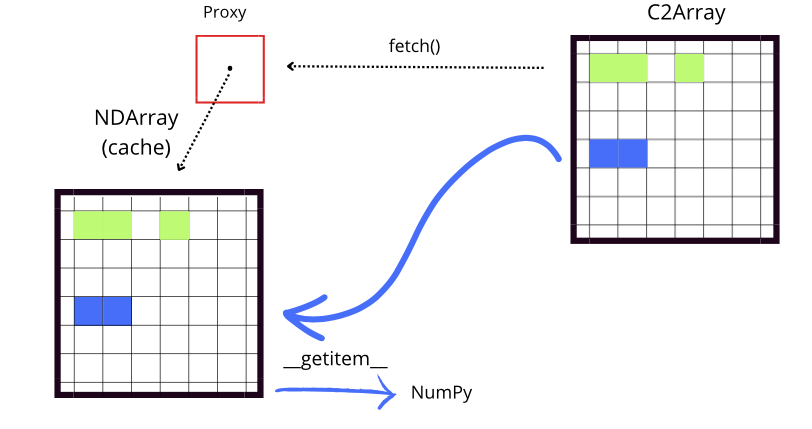
Fetching data with a Proxy

The fetch function is designed to return the local proxy, which serves as a cache for the requested data. This proxy, while representing the remote container, allows only a portion of the data to be initialized, with the rest potentially remaining empty or undefined (e.g., slice_data[1:3, 1:3]).

In this way, fetch downloads only the specific data that is required, which reduces the amount of data stored locally and optimizes the use of resources. This method is particularly useful when working with large datasets, as it allows for the efficient handling of multidimensional data.

# Fetch a slice of the data from the proxy
t0 = time.time()
slice_data = proxy.fetch(slice(0, 2))
t1 = time.time() - t0
print(f"Time to fetch: {t1:.2f} s")
print(f"File size after fetch (2 chunks): {get_file_size(local_path):.2f} MB")
print(slice_data[1:3, 1:3])

Time to fetch: 1.49 s
File size after fetch (2 chunks): 1.28 MB
[[[15712 13933 18298 ... 21183 22486 20541]
  [18597 21261 23925 ... 22861 21008 19155]]

 [[    0     0     0 ...     0     0     0]
  [    0     0     0 ...     0     0     0]]]

Above, using the fetch function with a slice involves downloading data from a chunk that had not been previously requested. This can lead to an increase in the local file size as new data is loaded.

In the previous result, only 2 chunks have been downloaded and initialized, which is reflected in the array with visible numerical values, as seen in the section [[15712 13933 18298 ... 21183 22486 20541], [18597 21261 23925 ... 22861 21008 19155]]. These represent data that are ready to be processed. On the other hand, the lower part of the array, [[0 0 0 ... 0 0 0], [0 0 0 ... 0 0 0]], shows an uninitialized section (normally filled with zeros).

This indicates that those chunks have not yet been downloaded or processed. The fetch function could eventually fill these chunks with data when requested, replacing the zeros (which indicate uninitialized data) with the corresponding values:

# Fetch a slice of the data from the proxy
t0 = time.time()
slice_data2 = proxy.fetch((slice(2, 3), slice(6, 7)))
t1 = time.time() - t0
print(f"Time to fetch: {t1:.2f} s")
print(f"File size after fetch (1 chunk): {get_file_size(local_path):.2f} MB")
print(slice_data[1:3, 1:3])

Time to fetch: 0.93 s
File size after fetch (1 chunk): 1.92 MB
[[[15712 13933 18298 ... 21183 22486 20541]
  [18597 21261 23925 ... 22861 21008 19155]]

 [[16165 14955 19889 ... 21203 22518 20564]
  [18610 21264 23919 ... 20509 19364 18219]]]

Now the fetch function has downloaded another two additional chunks, which is reflected in the local file size. The print show how all the slice [1:3, 1:3] has been initialized with data, while the rest of the array may remain uninitialized.

Data access using __getitem__

The __getitem__ function in the Proxy class is similar to fetch in that it allows for the retrieval of specific data from the remote container. However, __getitem__ returns a NumPy array, which can be used to access specific subsets of the data.

# Using __getitem__ to get a slice of the data
t0 = time.time()
result = proxy[5:7, 1:3]
t1 = time.time() - t0
print(f"Proxy __getitem__ time: {t1:.3f} s")
print(result)
print(type(result))
print(f"File size after __getitem__ (2 chunks): {get_file_size(local_path):.2f} MB")

Proxy __getitem__ time: 1.611 s
[[[16540 15270 20144 ... 20689 21494 19655]
  [17816 21097 24378 ... 21449 20582 19715]]

 [[16329 14563 18940 ... 20186 20482 19166]
  [17851 21656 25461 ... 23705 21399 19094]]]
<class 'numpy.ndarray'>
File size after __getitem__ (2 chunks): 3.20 MB

See? New data has been downloaded and initialized, as shown by the array values and the size of the local file. The __getitem__ function has accessed the data in the chunks, and put the slice in the result array, which is now available for processing. The local file size has increased due to the new data that has been downloaded and stored in the cache.

Differences between fetch and __getitem__

Although fetch and __getitem__ have distinct functions, they work together to facilitate efficient access to data. fetch manages the loading of data into the local cache by checking if the necessary chunks are available. If they are not, it downloads them from the remote source for future access.

On the other hand, __getitem__ handles the indexing and retrieval of data through a NumPy array, allowing access to specific subsets. Before accessing the data, __getitem__ calls fetch to ensure that the necessary chunks are in the cache. If the data is not present in the cache, fetch takes care of downloading it from its original location (for example, from disk or an external source). This ensures that when __getitem__ performs the indexing operation, it has immediate access to the data without interruptions.

An important detail is that, while both fetch and getitem ensure the necessary data is available, they may download more information than required because they download entire chunks. However, this can be advantageous when accessing large remote arrays, as it avoids downloading the whole dataset at once.

About the remote dataset

The remote dataset is available at: https://demo.caterva2.net/roots/example/lung-jpeg2000_10x.b2nd?roots=example. You may want to explore the data values by clicking on the Data tab; this dataset is actually a tomography of a lung, which you can visualize by clicking on the Tomography tab. Finally, by clicking on the Download button, it can be downloaded locally in case you want to experiment more with the data.

As we have seen, every time that we dowloaded a chunk, the size of the local file increased by a fix amount (around 0.64 MB). This is because the chunks (whose size is around 6.4 MB) are compressed with the Codec.GROK codec, which has been configured to reduce the size of the data by a constant factor of 10. This means that the compressed data occupies only one-tenth of the space that it would occupy without compression. This reduction in data size optimizes both storage and transfer, as data is always handled in a compressed state when downloading or storing images, which accelerates the transfer process.

Conclusion

This tutorial has highlighted how the efficient integration of the Proxy class in Blosc2, combined with the fetch and __getitem__ functions, optimizes access to multidimensional data. This combination of techniques not only enables the handling of large volumes of information more agilely, but also maximizes storage and processing resources, which is crucial in data-intensive environments and in scientific or industrial applications that require high efficiency and performance.