Matrix transposition is more than a textbook exercise, it plays a key role in memory-bound operations where layout and access patterns can make or break performance.

When working with large datasets, efficient data transformation can significantly improve both performance and compression ratios. In Blosc2, we recently implemented a matrix transposition function, a fundamental operation that rearranges data by swapping rows and columns. In this post, I'll share the design insights, implementation details, performance considerations that went into this feature, and an unexpected NumPy behaviour.

How it works

The following image illustrates the core idea behind matrix transposition in Blosc2:

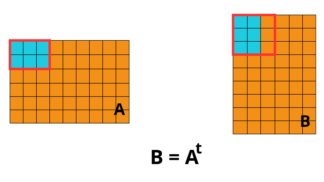
On the left, we have matrix A, and on the right, its transpose B = Aᵗ. Transposition means that an element located at position A[i][j] is moved to position B[j][i].

Each element in matrix A is shown as a colored cell, visually, the 2×3 blue chunk in A gets rotated and repositioned in B, illustrating how entire blocks of data shift when the matrix is transposed.

The red border marks the original chunk in both matrices. What’s interesting is that the shape of the chunks themselves changes during transposition. While A may use a 2×3 chunk layout, the transposed matrix B ends up with a different chunk geometry due to the new memory layout.

Why does this matter? In Blosc2, chunks define how data is split and compressed. Choosing the right chunk shape can drastically influence compression efficiency and decompression speed. So, understanding how chunks shift during operations like transposition is essential for optimizing performance.

Performance benchmark: Transposing matrices with Blosc2 vs NumPy

To evaluate the performance of the new matrix transposition implementation in Blosc2, I conducted a series of benchmarks comparing it to NumPy, which serves as the baseline due to its widespread use and high optimization level. The goal was to observe how both approaches perform when handling matrices of increasing size and to understand the impact of different chunk configurations in Blosc2.

Benchmark setup

All tests were conducted using matrices filled with float64 values, covering a wide range of sizes, starting from small 100×100 matrices and scaling up to very large matrices of size 17000×17000, covering data sizes from just a few megabytes to over 2 GB. Each matrix was transposed using the Blosc2 API under different chunking strategies:

In the case of NumPy, I used the .transpose() function followed by a .copy() to ensure that the operation was comparable to that of Blosc2. This is because, by default, NumPy's transposition is a view operation that only modifies the array's metadata, without actually rearranging the data in memory. Adding .copy() forces NumPy to perform a real memory reordering, making the comparison with Blosc2 fair and accurate.

For Blosc2, I tested the transposition function across several chunk configurations. Specifically, I included:

Automatic chunking (None), where Blosc2 decides the optimal chunk size internally.
Fixed chunk sizes: (150, 300), (500, 200), (1000, 1000) and (5000, 5000).

These chunk sizes were chosen to represent a mix of square and rectangular blocks, allowing me to study how chunk geometry impacts performance, especially for very large matrices.

Each combination of library and configuration was tested across all matrix sizes, and the time taken to perform the transposition was recorded in seconds. This comprehensive setup makes it possible to compare not just raw performance, but also how well each method scales with data size and structure.

Results and discussion

The chart below summarizes the benchmark results for matrix transposition using NumPy and Blosc2, across various chunk shapes and matrix sizes.

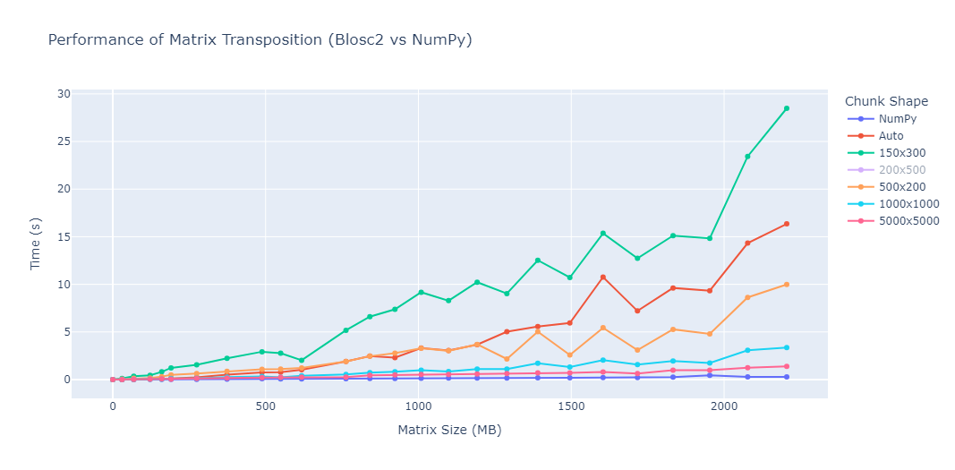
While NumPy sets a strong performance baseline, the behaviour of Blosc2 becomes particularly interesting when we dive into how different chunk configurations affect transposition speed. The following observations highlight how crucial the choice of chunk shape is to achieving optimal performance.

Large, square chunks such as (1000, 1000) and (5000, 5000) offered the fastest and most stable transpositions, keeping execution times below 3 seconds even for matrices exceeding 2 GB. These shapes minimize chunk overhead and maximize cache locality, which is key to achieving high throughput in Blosc2.
Automatic chunking also performs reasonably well, though its timings fluctuate more as matrix sizes increase. It appears that while the automatic mode is generally robust, it doesn't always choose optimal chunk boundaries, especially for very large arrays, which can lead to inconsistent transposition speeds.
Small rectangular chunks show the poorest performance, with transposition times skyrocketing for large matrices. For example, (150, 300) reaches nearly 30 seconds at around 2200 MB of matrix size, about 100× slower than NumPy. This is likely due to poor cache utilization and increased overhead in managing a high number of small blocks.

These benchmarks confirm that chunk configuration plays a critical role in how well Blosc2 performs. Unlike traditional in-memory libraries, Blosc2’s behaviour can vary greatly depending on how data is internally structured.

Conclusion

The benchmarks highlight one key insight: Blosc2 is highly sensitive to chunk shape, and its performance can range from excellent to poor depending on how it is configured. With the right chunk size, Blosc2 can offer both high-speed transpositions and advanced features like compression and out-of-core processing. However, misconfigured chunks, especially those that are too small or uneven, can drastically reduce its effectiveness. This makes chunk tuning an essential step for anyone seeking to get the most out of Blosc2 for large-scale matrix operations.

Appendix: Unexpected behaviour in NumPy

While running the benchmarks, two unusual spikes were consistently observed in the performance of NumPy around matrices of approximately 500 MB, 1100 MB and 1900 MB in size. This can be clearly seen in the plot below:

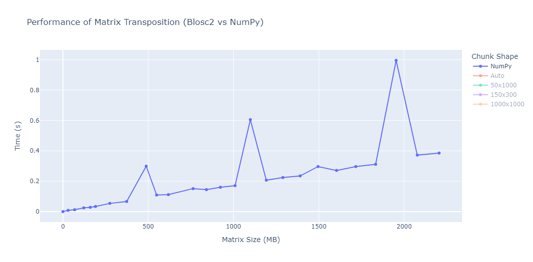
This sudden increase in transposition time is consistently reproducible and does not seem to correlate with the gradual increase expected from larger memory sizes. We have also observed this behaviour in other machines, although at different sizes.

This observation reinforces the importance of testing under realistic and varied conditions, as performance is not always linear or intuitive.