Peaking compression performance in PyTables with direct chunking

Using the API

The direct chunking API consists of three operations: get information about a chunk (chunk_info()), write a raw chunk (write_chunk()), and read a raw chunk (read_chunk()). They are supported by chunked datasets (CArray, EArray and Table), i.e. those whose data is split into fixed-size chunks of the same dimensionality as the dataset (maybe padded at its boundaries), with HDF5 pipeline filters like compressors optionally processing them on read/write.

chunk_info() returns an object with useful information about the chunk containing the item at the given coordinates. Let's create a simple 100x100 array with 10x100 chunks compressed with Blosc2+LZ4 and get info about a chunk:

>>> import tables, numpy
>>> h5f = tables.open_file('direct-example.h5', mode='w')
>>> filters = tables.Filters(complib='blosc2:lz4', complevel=2)
>>> data = numpy.arange(100 * 100).reshape((100, 100))
>>> carray = h5f.create_carray('/', 'carray', chunkshape=(10, 100),
                               obj=data, filters=filters)
>>> coords = (42, 23)
>>> cinfo = carray.chunk_info(coords)
>>> cinfo
ChunkInfo(start=(40, 0), filter_mask=0, offset=6779, size=608)

So the item at coordinates (42, 23) is stored in a chunk of 608 bytes (compressed) which starts at coordinates (40, 0) in the array and byte 6779 in the file. The latter offset may be used to let other code access the chunk directly on storage. For instance, since Blosc2 was the only HDF5 filter used to process the chunk, let's open it directly:

>>> import blosc2
>>> h5f.flush()
>>> b2chunk = blosc2.open(h5f.filename, mode='r', offset=cinfo.offset)
>>> b2chunk.shape, b2chunk.dtype, data.itemsize
((10, 100), dtype('V8'), 8)

Since Blosc2 does understand the structure of data (thanks to b2nd), we can even see that the chunk shape and the data item size are correct. The data type is opaque to the HDF5 filter which wrote the chunk, hence the V8 dtype. Let's check that the item at (42, 23) is indeed in that chunk:

>>> chunk = numpy.ndarray(b2chunk.shape, buffer=b2chunk[:],
                          dtype=data.dtype)  # Use the right type.
>>> ccoords = tuple(numpy.subtract(coords, cinfo.start))
>>> bool(data[coords] == chunk[ccoords])
True

This offset-based access is actually what b2nd optimized slicing performs internally. Please note that neither PyTables nor HDF5 were involved at all in the actual reading of the chunk (Blosc2 just got a file name and an offset). It's difficult to cut more overhead than that!

It won't always be the case that you can (or want to) read a chunk in that way. The read_chunk() method allows you to read a raw chunk as a new byte string or into an existing buffer, given the chunk's start coordinates (which you may compute yourself or get via chunk_info()). Let's use read_chunk() to redo the reading that we just did above:

>>> rchunk = carray.read_chunk(coords)
Traceback (most recent call last):
    ...
tables.exceptions.NotChunkAlignedError: Coordinates are not multiples
    of chunk shape: (42, 23) !* (np.int64(10), np.int64(100))
>>> rchunk = carray.read_chunk(cinfo.start)  # Always use chunk start!
>>> b2chunk = blosc2.ndarray_from_cframe(rchunk)
>>> chunk = numpy.ndarray(b2chunk.shape, buffer=b2chunk[:],
                          dtype=data.dtype)  # Use the right type.
>>> bool(data[coords] == chunk[ccoords])
True

The write_chunk() method allows you to write a byte string into a raw chunk. Please note that you must first apply any filters manually, and that you can't write chunks beyond the dataset's current shape. However, remember that enlargeable datasets may be grown or shrunk in an efficient manner using the truncate() method, which doesn't write new chunk data. Let's use that to create an EArray with the same data as the previous CArray, chunk by chunk:

>>> earray = h5f.create_earray('/', 'earray', chunkshape=carray.chunkshape,
                               atom=carray.atom, shape=(0, 100),  # Empty.
                               filters=filters)  # Just to hint readers.
>>> earray.write_chunk((0, 0), b'whatever')
Traceback (most recent call last):
    ...
IndexError: Chunk coordinates not within dataset shape:
    (0, 0) <> (np.int64(0), np.int64(100))
>>> earray.truncate(len(carray))  # Grow the array (cheaply) first!
>>> for cstart in range(0, len(carray), carray.chunkshape[0]):
...     chunk = carray[cstart:cstart + carray.chunkshape[0]]
...     b2chunk = blosc2.asarray(chunk)  # May be customized.
...     wchunk = b2chunk.to_cframe()  # Serialize.
...     earray.write_chunk((cstart, 0), wchunk)

You can see that such low-level writing is more involved than usual. Though we used default Blosc2 parameters here, the explicit compression step allows you to fine-tune it in ways not available through PyTables like setting internal chunk and block sizes or even using Blosc2 compression plugins like Grok/JPEG2000. In fact, the filters given on dataset creation are only used as a hint, since each Blosc2 container holding a chunk includes enough metadata to process it independently. In the example, the default chunk compression parameters don't even match dataset filters (using Zstd instead of LZ4):

>>> carray.filters
Filters(complevel=2, complib='blosc2:lz4', ...)
>>> earray.filters
Filters(complevel=2, complib='blosc2:lz4', ...)
>>> b2chunk.schunk.cparams['codec']
<Codec.ZSTD: 5>

Still, the Blosc2 HDF5 filter plugin included with PyTables is able to read the data just fine:

>>> bool((carray[:] == earray[:]).all())
True
>>> h5f.close()

You may find a more elaborate example of using direct chunking in PyTables' examples.

Benchmarks

b2nd optimized slicing shows us that removing the HDF5 filter pipeline from the I/O path can result in sizable performance increases, if the right chunking and compression parameters are chosen. To check the impact of using the new direct chunking API, we ran some benchmarks that compare regular and direct read/write speeds. On an AMD Ryzen 7 7800X3D CPU with 8 cores, 96 MB L3 cache and 8 MB L2 cache, clocked at 4.2 GHz, we got the following results:

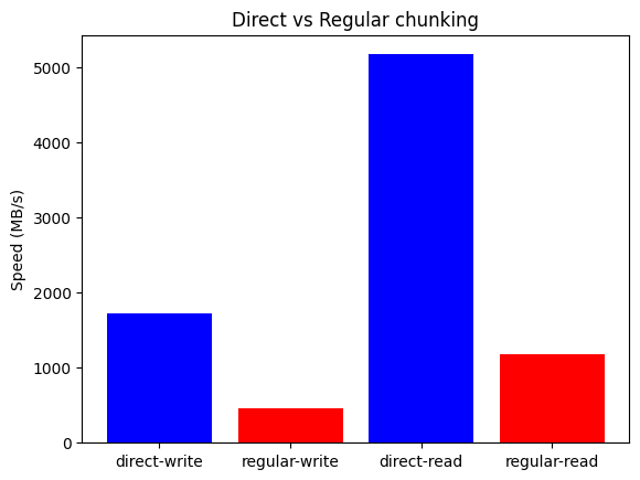
We can see that direct chunking yields 3.75x write and 4.4x read speedups, reaching write/read speeds of 1.7 GB/s and 5.2 GB/s. These are quite impressive numbers, though the base equipment is already quite powerful. Thus we also tried the same benchmark on a consumer-level MacBook Air laptop with an Apple M1 CPU with 4+4 cores and 12 MB L2 cache, clocked at 3.2 GHz, with the following results:

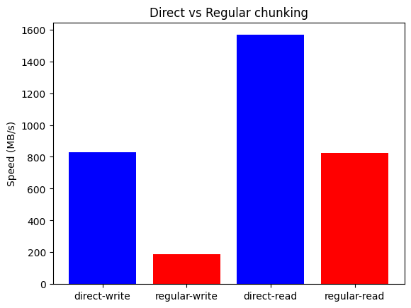
In this case direct chunking yields 4.5x write and 1.9x read speedups, with write/read speeds of 0.8 GB/s and 1.6 GB/s. The absolute numbers are of course not as impressive, but the performance is still much better than that of the regular mechanism, especially when writing. Please note that the M1 CPU has a hybrid efficiency+performance core configuration; as an aside, running the benchmark on a high-range Intel Core i9-13900K CPU also with a hybrid 8+16 core configuration (32 MB L2, 5.7 GHz) raised the write speedup to 4.6x, reaching an awesome write speed of 2.6 GB/s.

All in all, it's clear that bypassing the HDF5 filter pipeline results in immediate I/O speedups. You may find a Jupyter notebook with the benchmark code and AMD CPU data in PyTables' benchmarks.

Conclusions

First of all, we (Ivan Vilata and Francesc Alted) want to thank everyone who made this new 3.10 release of PyTables possible, especially Antonio Valentino for his role of project maintainer, and the many code and issue contributors. Trying the new direct chunking API is much easier because of them. And of course, a big thank you to the NumFOCUS Foundation for making this whole new feature possible by funding its development!

In this post we saw how PyTables' direct chunking API allows one to squeeze the extra drop of performance that the most demanding scenarios require, when adjusting chunking and compression parameters in PyTables itself can't go any further. Of course, its low-level nature makes its use less convenient and safe than higher-level mechanisms, so you should evaluate whether the extra effort pays off. If used carefully with robust filters like Blosc2, the direct chunking API should shine the most in the case of large datasets with sustained I/O throughput demands, while retaining compatibility with other HDF5-based tools.