Efficient array concatenation launched in Blosc2

Update (2025-06-23): Recently, Luke Shaw added a stack() function in Blosc2, using the concatenate feature described here. The new function allows you to stack arrays along a new axis, which is particularly useful for creating higher-dimensional arrays from lower-dimensional ones. We have added a section at the end of this post to show the usage and performance of this new function.

---

Blosc2 just got a cool new trick: super-efficient array concatenation! If you've ever needed to combine several arrays into one, especially when dealing with lots of data, this new feature is for you. It's built to be fast and use as little memory as possible. This is especially true if your array sizes line up nicely with Blosc2's internal "chunks" (think of these as the building blocks of your compressed data). When this alignment happens, concatenation is lightning-fast, making it perfect for demanding tasks.

You can use this new concatenate feature whether you're coding in C or Python, and it works with any Blosc2 NDArray (Blosc2's way of handling multi-dimensional arrays).

Let's see how easy it is to use in Python. If you're familiar with NumPy, the blosc2.concatenate function will feel very similar:

import blosc2
# Create some sample arrays
a = blosc2.full((10, 20), 1, urlpath="arrayA.b2nd", mode="w")
b = blosc2.full((10, 20), 2, urlpath="arrayB.b2nd", mode="w")
c = blosc2.full((10, 20), 3, urlpath="arrayC.b2nd", mode="w")
# Concatenate the arrays along the first axis
result = blosc2.concat([a, b, c], axis=0, urlpath="destination.b2nd", mode="w")
# The result is a new Blosc2 NDArray containing the concatenated data
print(result.shape)  # Output: (30, 20)
# You can also concatenate along other axes
result_axis1 = blosc2.concat([a, b, c], axis=1, urlpath="destination_axis1.b2nd", mode="w")
print(result_axis1.shape)  # Output: (10, 60)

The blosc2.concatenate function is pretty straightforward. You give it a list of the arrays you want to join together. You can also tell it which way to join them using the axis parameter (like joining them end-to-end or side-by-side).

A really handy feature is that you can use urlpath and mode to save the combined array directly to a file. This is great when you're working with huge datasets because you don't have to load everything into memory at once. What you get back is a brand new, persistent Blosc2 NDArray with all your data combined.

Aligned versus Non-Aligned Concatenation

Blosc2's concatenate function is smart. It processes your data in small pieces of compressed data (chunks). This has two consequences. The first is that you can join very large arrays, stored on your disk, chunk-by-chunk without using up all your computer's memory. Secondly, if the chunks fit neatly into the arrays to be concatenated, the process is much faster. Why? Because Blosc2 can avoid a lot of extra work, chiefly decompressing and re-compressing the chunks.

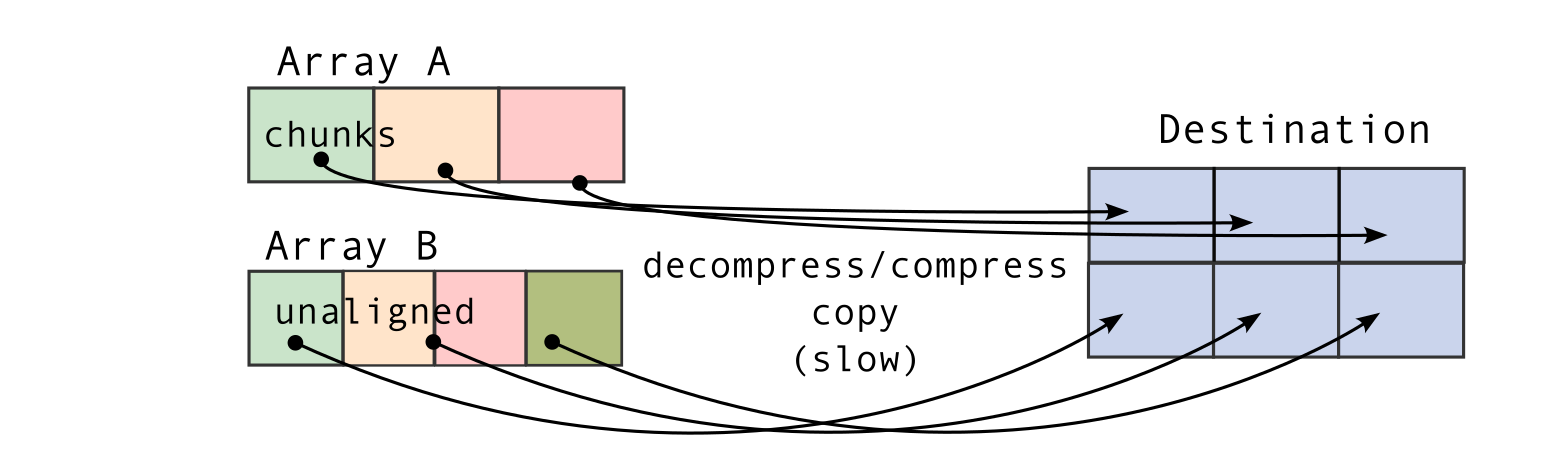
Let's look at some pictures to see what "aligned" and "unaligned" concatenation means. "Aligned" means that chunk boundaries of the arrays to be concatenated line up with each other. "Unaligned" means that this is not the case.
/images/blosc2-new-concatenate/concat-unaligned.png/images/blosc2-new-concatenate/concat-aligned.png

The pictures show why "aligned" concatenation is faster. In Blosc2, all data pieces (chunks) inside an array must be the same size. So, if the chunks in the arrays you're joining match up ("aligned"), Blosc2 can combine them very quickly. It doesn't have to rearrange the data into new, same-sized chunks for the final array. This is a big deal for large arrays.

If the arrays are "unaligned," Blosc2 has more work to do. It has to decompress and then re-compress the data to make the new chunks fit, which takes longer. There's one more small detail for this fast method to work: the first array's size needs to be a neat multiple of its chunk size along the direction you're joining.

A big plus with Blosc2 is that it always processes data in these small chunks. This means it can combine enormous arrays without ever needing to load everything into your computer's memory at once.

Performance

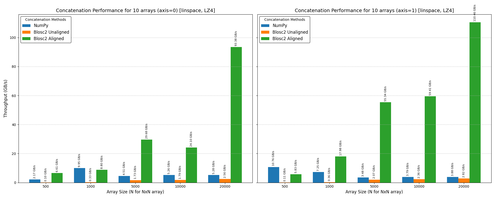
To show you how much faster this new concatenate feature is, we did a speed test using LZ4 as the internal compressor in Blosc2. We compared it to the usual way of joining arrays with numpy.concatenate.
/images/blosc2-new-concatenate/benchmark-lz4-20k-i13900K.png

The speed tests show that Blosc2's new concatenate is rather slow for small arrays (like 1,000 x 1,000). This is because it has to do a lot of work to set up the concatenation. But when you use larger arrays (like 20,000 x 20,000) that start to exceed the memory limits of our test machine (32 GB of RAM), Blosc2's new concatenate peformance is much better, and nearing the performance of NumPy's concatenate function.

However, if your array sizes line up well with Blosc2's internal chunks ("aligned" arrays), Blosc2 becomes much faster—typically more than 10x times faster than NumPy for large arrays. This is because it can skip a lot of the work of decompressing and re-compressing data, and the cost of copying compressed data is also lower (as much as the achieved compression ratio, which for this case is around 10x).

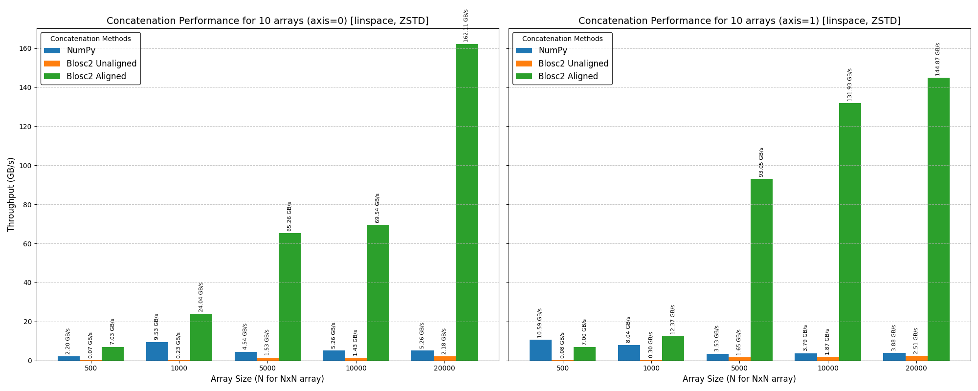
Using the Zstd compressor with Blosc2 can make joining "aligned" arrays even quicker, since Zstd is good at making data smaller.
/images/blosc2-new-concatenate/benchmark-zstd-20k-i13900K.png

So, when arrays are aligned, there's less data to copy (compression ratios here are around 20x), which speeds things up. If arrays aren't aligned, Zstd is a bit slower than the previous compressor (LZ4) because its decompression and re-compression algorithm is slower. Conclusion? Pick the compressor that works best for what you're doing!

Stacking Arrays

We've also added a new stack() function in Blosc2 that uses the concatenate feature. This function lets you stack arrays along a new axis, which is super useful for creating higher-dimensional arrays from lower-dimensional ones. Here's how it works:

import blosc2
# Create some sample arrays
a = blosc2.full((10, 20), 1, urlpath="arrayA.b2nd", mode="w")
b = blosc2.full((10, 20), 2, urlpath="arrayB.b2nd", mode="w")
c = blosc2.full((10, 20), 3, urlpath="arrayC.b2nd", mode="w")
# Stack the arrays along a new axis
stacked_result = blosc2.stack([a, b, c], axis=0, urlpath="stacked_destination.b2nd", mode="w")
print(stacked_result.shape)  # Output: (3, 10, 20)
# You can also stack along other axes
stacked_result_axis1 = blosc2.stack([a, b, c], axis=1, urlpath="stacked_destination_axis1.b2nd", mode="w")
print(stacked_result_axis1.shape)  # Output: (10, 3, 20)

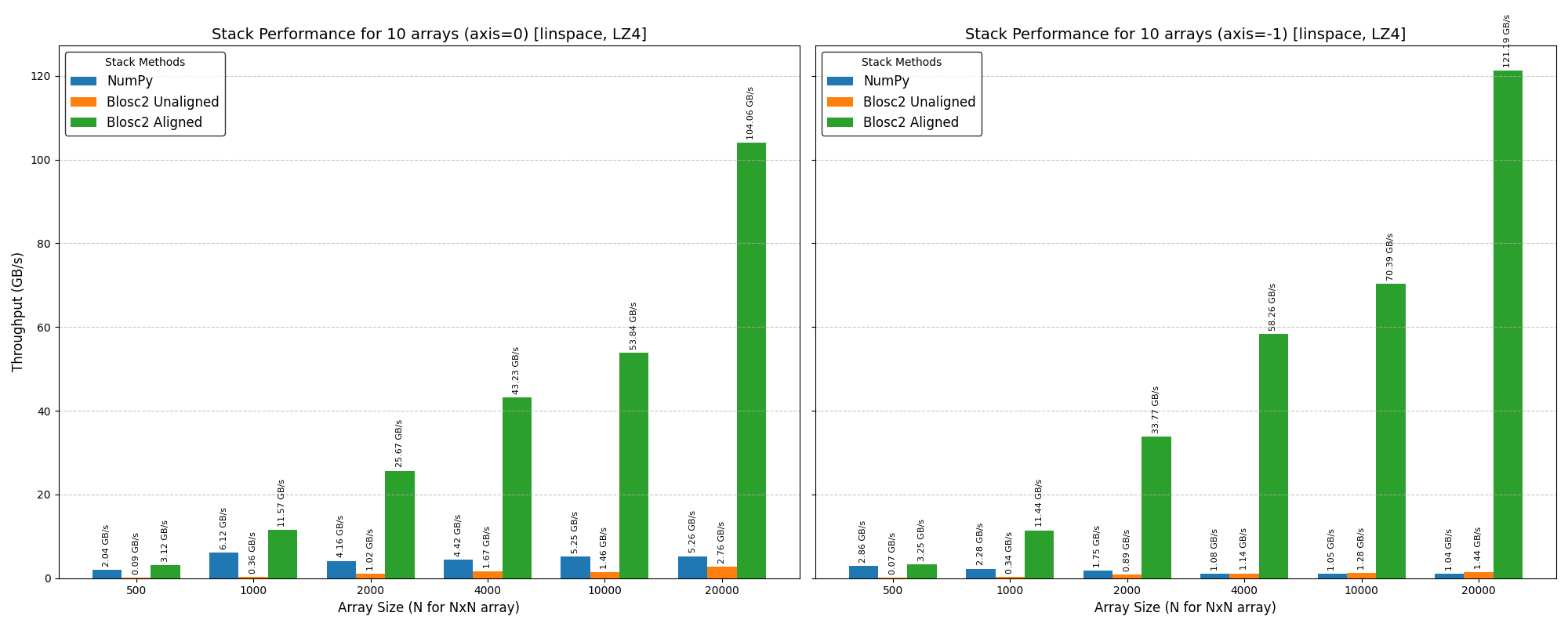
Benchmarks for the stack() function show that it performs similarly to the concat() function, especially when the input arrays are aligned. Here are the results for the same data sizes and machine used in the previous benchmarks, and using the LZ4 compressor.
/images/blosc2-new-concatenate/stack-lz4-20k-i13900K.png

And here are the results for the Zstd compressor.
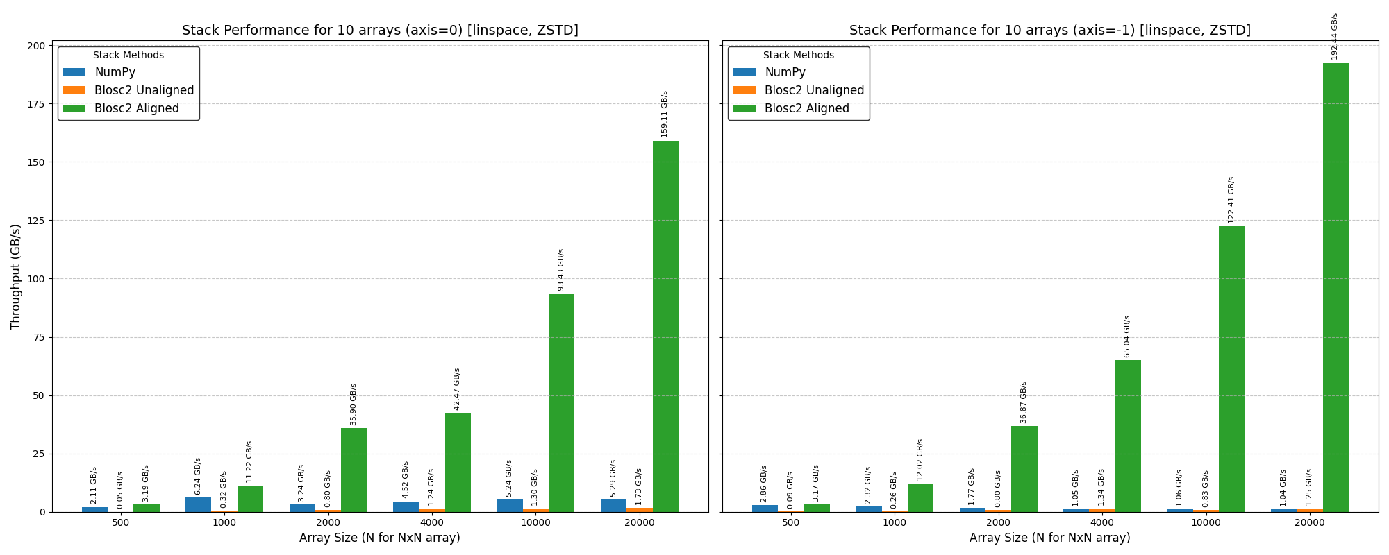
/images/blosc2-new-concatenate/stack-zstd-20k-i13900K.png

As can be seen, the stack() function is also very fast when the input arrays are aligned, and it performs well even for large arrays that don't fit into memory. Incidentally, when using the blosc2.stack() function in the last dim, it is slightly faster than numpy.stack() even when the arrays are not aligned; we are not sure why this is the case, but the fact that we can reproduces this behaviour is probably a sign that NumPy can optimize this use case better.

Conclusion

Blosc2's new concatenate and stack features are a great way to combine arrays quickly and without using too much memory. They are especially fast when your array sizes are an exact multiple of Blosc2's "chunks" (aligned arrays), making it perfect for big data jobs. They also work well for large arrays that don't fit into memory, as it processes data in small chunks. Finally, they are supported in both C and Python, so you can use them in your favorite programming language.

Give it a try in your own projects! If you have questions, the Blosc2 community is here to help.

If you appreciate what we're doing with Blosc2, please think about supporting us. Your help lets us keep making these tools better.
Make NDArray Transposition Fast (and Compressed!) within Blosc 2

Update (2025-04-30): The transpose function is now officially deprecated and replaced by the new permute_dims. This transition follows the Python array API standard v2022.12, aiming to make Blosc2 even more compatible with modern Python libraries and workflows.

In contrast with the previous transpose, the new permute_dims offers:

  • Support for arrays of any number of dimensions.

  • Full handling of arbitrary axis permutations, including support for negative indices.

Moreover, I have found a new way to transpose matrices more efficiently for Blosc2. This blog contains updated plots and discussions.

---

Matrix transposition is more than a textbook exercise, it plays a key role in memory-bound operations where layout and access patterns can make or break performance.

When working with large datasets, efficient data transformation can significantly improve both performance and compression ratios. In Blosc2, we recently implemented a matrix transposition function, a fundamental operation that rearranges data by swapping rows and columns. In this post, I'll share the design insights, implementation details, performance considerations that went into this feature, and an unexpected NumPy behaviour.

What was the old behavior?

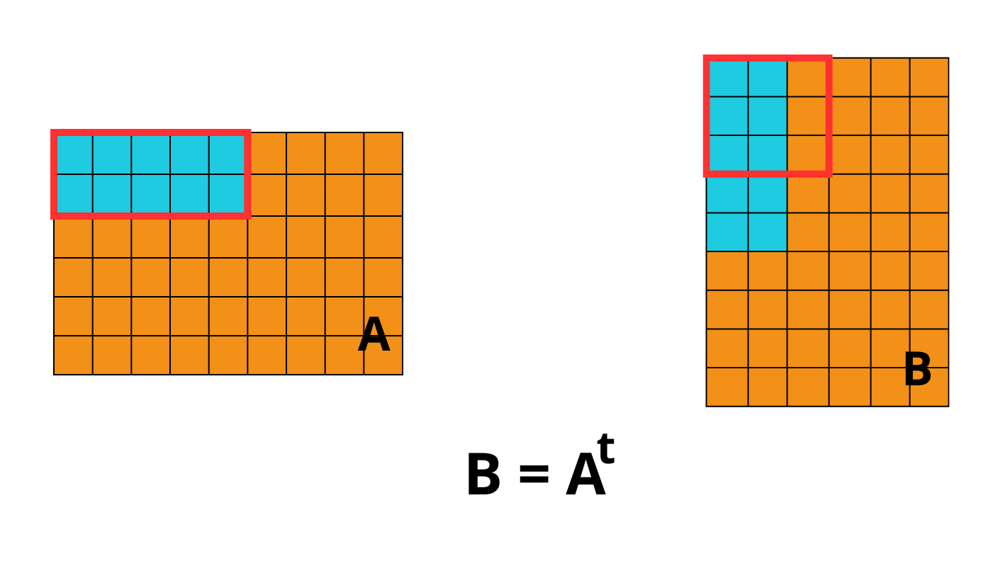
Previously, calling blosc2.transpose(A) would transpose the data within each chunk, and a new chunk shape would be chosen for the output array. However, this new chunk shape was not necessarily aligned with the new memory access patterns induced by the transpose. As a result, even though the output looked correct, accessing data along the new axes still incurred a significant overhead due to increased number of I/O operations. This lead to performance bottlenecks, particularly in workloads that rely on efficient memory access patterns.

Transposition explanation for old operation

What's new?

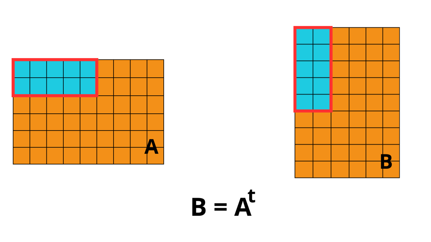
The permute_dims function in Blosc2 has been redesigned to greatly improve performance when working with compressed, multidimensional arrays. The main improvement lies in transposing the chunk layout alongside the array data, which eliminates the overhead of cross-chunk access patterns.

The new implementation transposes the chunk layout along with the data. For example, an array with chunks=(2, 5) that is transposed with axes=(1, 0) will result in an array with chunks=(5, 2). This ensures that the output layout matches the new data order, making block access contiguous and efficient.

This logic generalizes to N-dimensional arrays and applies regardless of their shape or chunk configuration.

Transposition explanation for new operation

Performance benchmark: Transposing matrices with Blosc2 vs NumPy

To evaluate the performance of the new matrix transposition implementation in Blosc2, I conducted a series of benchmarks comparing it to NumPy, which serves as the baseline due to its widespread use and high optimization level. The goal was to observe how both approaches perform when handling matrices of increasing size and to understand the impact of different chunk configurations in Blosc2.

Benchmark setup

All tests were conducted using matrices filled with float64 values, covering a wide range of sizes, starting from small 100×100 matrices and scaling up to very large matrices of size 17000×17000, covering data sizes from just a few megabytes to over 2 GB. Each matrix was transposed using the Blosc2 API under different chunking strategies:

In the case of NumPy, I used the .transpose() function followed by a .copy() to ensure that the operation was comparable to that of Blosc2. This is because, by default, NumPy's transposition is a view operation that only modifies the array's metadata, without actually rearranging the data in memory. Adding .copy() forces NumPy to perform a real memory reordering, making the comparison with Blosc2 fair and accurate.

For Blosc2, I tested the transposition function across several chunk configurations. Specifically, I included:

  • Automatic chunking, where Blosc2 decides the optimal chunk size internally.

  • Fixed chunk sizes: (150, 300), (1000, 1000) and (5000, 5000).

These chunk sizes were chosen to represent a mix of square and rectangular blocks, allowing me to study how chunk geometry impacts performance, especially for very large matrices.

Each combination of library and configuration was tested across all matrix sizes, and the time taken to perform the transposition was recorded in seconds. This comprehensive setup makes it possible to compare not just raw performance, but also how well each method scales with data size and structure.

Results and discussion

The chart below summarizes the benchmark results for matrix transposition using NumPy and Blosc2, across various chunk shapes and matrix sizes.

Transposition performance for new method

While NumPy sets a strong performance baseline, the behaviour of Blosc2 becomes particularly interesting when we dive into how different chunk configurations affect transposition speed. The following observations highlight how crucial the choice of chunk shape is to achieving optimal performance.

  • Large square chunks (e.g., (4000, 4000)) showed the worst performance, especially with large matrices. Despite having fewer chunks, their size seems to hinder cache performance and introduces memory pressure that degrades throughput. Execution times were consistently higher than other configurations.

  • Small rectangular chunks such as (150, 300) also underperformed. As matrix size grew, execution times increased significantly, reaching nearly 3 seconds at around 2200 MB, likely due to poor cache utilization and the overhead of managing many tiny chunks.

  • Mid-sized square chunks like (1000, 1000) delivered consistently solid results across all tested sizes. Their timings stay below ~1.2 s with minimal variance, making them a reliable manual choice.

  • Automatically selected chunks consistently achieved the best performance. By adapting chunk layout to the data shape and size, the internal heuristics outpaced all fixed configurations, even rivaling plain NumPy transpose times.

Blosc2 vs NumPy comparison

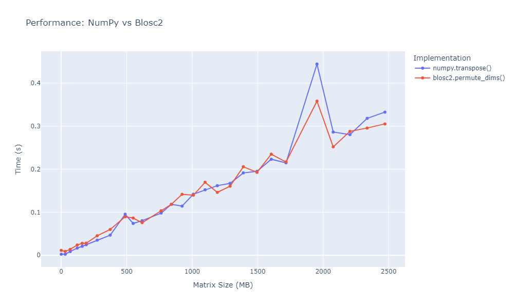
The second plot provides a direct comparison between the standard NumPy transpose and the newly optimized Blosc2 version. It shows that Blosc2’s optimized implementation closely matches NumPy's performance, even for larger matrices. The results confirm that with good chunking strategies and proper memory handling, Blosc2 can achieve performance on par with NumPy for transposition operations.

Conclusion

The benchmarks highlight one key insight: Blosc2 is highly sensitive to chunk shape, and its performance can range from excellent to poor depending on how it is configured. With the right chunk size, Blosc2 can offer both high-speed transpositions and advanced features like compression and out-of-core processing. However, misconfigured chunks, especially those that are too big or too small, can drastically reduce its effectiveness. This makes chunk tuning an essential step for anyone seeking to get the most out of Blosc2 for large-scale matrix operations.

Appendix A: Unexpected NumPy behaviour

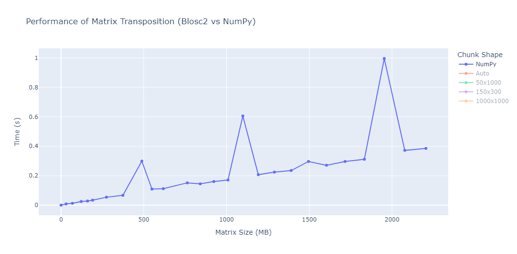
While running the benchmarks, two unusual spikes were consistently observed in the performance of NumPy around matrices of approximately 500 MB, 1100 MB and 2000 MB in size. This can be clearly seen in the plot below:

NumPy transposition performance anomaly

This sudden increase in transposition time is consistently reproducible and does not seem to correlate with the gradual increase expected from larger memory sizes. We have also observed this behaviour in other machines, although at different sizes.

This observation reinforces the importance of testing under realistic and varied conditions, as performance is not always linear or intuitive.

Optimizing chunks for matrix multiplication in Blosc2

As data volumes continue to grow in fields like machine learning and scientific computing, optimizing fundamental operations like matrix multiplication becomes increasingly critical. Blosc2's chunk-based approach offers a new path to efficiency in these scenarios.

Matrix Multiplication

Matrix multiplication is a fundamental operation in many scientific and engineering applications. With the introduction of matrix multiplication into Blosc2, users can now perform this operation on compressed arrays efficiently. The key advantages of having matrix multiplication in Blosc2 include:

  • Compressed matrices in memory: Blosc2 enables matrices to be stored in a compressed format without sacrificing the ability to perform operations directly on them.

  • Efficiency with chunks: In computation-intensive applications, matrix multiplication can be executed without fully decompressing the data, operating on small blocks of data independently, saving both time and memory.

  • Out-of-core computation: When matrices are too large to fit in main memory, Blosc2 facilitates out-of-core processing. Data stored on disk is read and processed in optimized chunks, allowing matrix multiplication operations without loading the entire dataset into memory.

These features are especially valuable in big data environments and in scientific or engineering applications where matrix sizes can be overwhelming, enabling complex calculations efficiently.

Implementation

The matrix multiplication functionality is implemented in the matmul function. It supports Blosc2 NDArray objects and leverages chunked operations to perform the multiplication efficiently.

How blocked matrix multiplication works

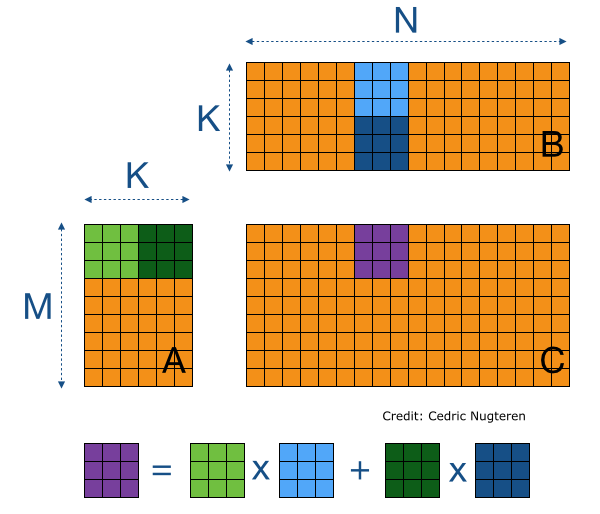
The image illustrates a blocked matrix multiplication approach. The key idea is to divide matrices into smaller blocks (or chunks) to optimize memory access and computational efficiency.

In the image, matrix A (M x K) and matrix B (K x N) are partitioned into chunks, and these are partitioned into blocks. The resulting matrix C (M x N) is computed as a sum of block-wise multiplication.

This method significantly improves cache utilization by ensuring that only the necessary parts of the matrices are loaded into memory at any given time. In Blosc2, storing matrix blocks as compressed chunks reduces memory footprint and enhances performance by enabling on-the-fly decompression.

Also, Blosc2 supports a wide range of data types. In addition to standard Python types such as int, float, and complex, it also fully supports various NumPy types. The currently supported types include:

  • np.int8

  • np.int16

  • np.int32

  • np.int64

  • np.float32

  • np.float64

  • np.complex64

  • np.complex128

This versatility allows compression and subsequent processing to be applied across diverse scenarios, tailored to the specific needs of each application.

Together, these features make Blosc2 a flexible and adaptable tool for various scenarios, but especially suited for the handling of large datasets.

Benchmarks

The benchmarks have been designed to evaluate the performance of the matmul function under various conditions. Here are the key aspects of our experimental setup and findings:

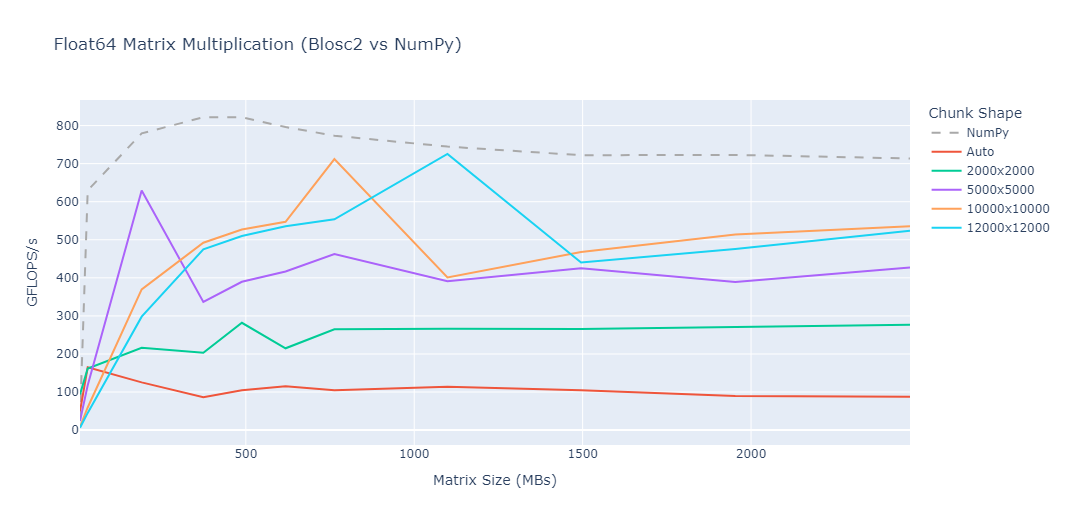
Different matrix sizes were tested using both float32 and float64 data types. All the matrices used for multiplication are square. The variation in matrix sizes helps observe how the function scales and how the overhead of chunk management impacts performance.

The x-axis represents the size of the resulting matrix in megabytes (MB). We used GFLOPS (Giga Floating-Point Operations per Second) to gauge the computational throughput, allowing us to compare the efficiency of the matmul function relative to highly optimized libraries like NumPy.

Blosc2 also incorporates a functionality to automatically select chunks, and it is represented in the benchmark by "Auto".

Benchmark float32Benchmark float64

For smaller matrices, the overhead of managing chunks in Blosc2 can result in lower GFLOPS compared to NumPy. As the matrix size increases, Blosc2 scales well, approaching its performance to NumPy.

Each chunk shape exhibits a peak performance when the matrix size matches the chunk size, or is a multiple of the chunk shape.

Conclusion

The new matrix multiplication feature in Blosc2 introduces efficient, chunked computation for compressed arrays. This allows users to handle large datasets both in memory and on disk without sacrificing performance. The implementation supports a wide range of data types, making it versatile for various numerical applications.

Real-world applications, such as neural network training, demonstrate the potential benefits in scenarios where memory constraints and large data sizes are common. While there are some limitations —such as support only for 2D arrays and the overhead of blocking— the applicability looks promising, like potential integration with deep learning frameworks.

Overall, Blosc2 offers a compelling alternative for applications where the advantages of compression and out-of-core computation are critical, paving the way for more efficient processing of massive datasets.

Getting my feet wet with Blosc2

In the initial phase of the project, my biggest challenge was understanding how Blosc2 manages data internally. For matrix multiplication, it was critical to grasp how to choose the right chunks, since the operation requires that the ranges of both matrices coincide. After some considerations and a few insightful conversations with Francesc, I finally understood the underlying mechanics. This breakthrough allowed me to begin implementing the first versions of my solution, adjusting the data fragmentation so that each block was properly aligned for precise computation.

Another important aspect was adapting to the professional workflow of using Git for version control. Embracing Git —with its branch creation, regular commits, and conflict resolution— represented a significant shift in my development approach. This experience not only improved the organization of my code and facilitated collaboration but also instilled a structured and disciplined mindset in managing my projects. This tool has shown to be both valuable and extremely helpful.

Finally, the moment when the function finally returned the correct result was really exciting. After multiple iterations, the rigorous debugging process paid off as everything fell into place. This breakthrough validated the robustness of the implementation and boosted my confidence to further optimize and tackle new challenges in data processing.